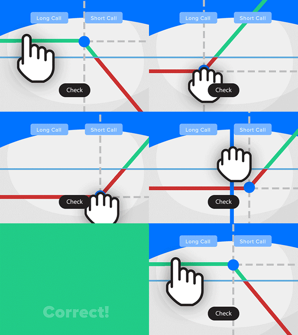
- Solve real problems with our hands-on interface
- Progress from basic puts and calls to advanced strategies
Interactive Options Course

Posted August 10, 2026 at 12:55 pm

The article “Process Large Financial Datasets With PySpark And Python” was originally published on PyQuant News.
This PySpark tutorial shows how to work with financial datasets that are too large for pandas (a popular Python library for table-shaped data) to handle on one machine. If you’re doing data analysis with Python and your files have grown past a few gigabytes, PySpark lets you process them across multiple CPU cores or machines using familiar Python syntax. This guide shows how to install PySpark and load market data. Then you’ll run a few common operations. If you’re newer to Python, the getting started with Python for quant finance guide covers the fundamentals.
PySpark lets you control Apache Spark, an open-source engine for big data processing, from Python. Spark breaks a large dataset into smaller pieces, runs the same operation on each piece, and then combines the results. In the most common workflow, pandas reads an entire file into one machine’s memory (RAM, your computer’s short-term working space), while Spark is built to split the work across many pieces of data. This matters when you’re dealing with millions of rows of trade-by-trade price data or large options tables that list contracts across many strike prices and expiration dates.
Pandas works well for datasets that fit in your computer’s RAM. Financial data grows fast, though. A single year of minute-level price data for 500 stocks can exceed 10 GB, and options data runs even larger.
PySpark handles this by distributing data across partitions, which are chunks of the dataset processed separately. Spark can send different partitions to different CPU cores, which is how it speeds up large jobs. You write Python code that looks similar to pandas, and Spark figures out how to split the work.
We’ll use stock trade data below so you can see what these operations look like on a realistic dataset.
You can install PySpark with pip. It includes a local Spark setup, so you don’t need a separate cluster of machines to get started.
pip install pyspark
If Spark doesn’t start after installation, check that Java is installed and available on your system. Spark depends on Java, and missing it is the most common setup failure.
Every PySpark program starts by creating a SparkSession, which is the main object you use to load data, run queries, and create Spark DataFrames (table-like structures similar to pandas, but designed to run across multiple machines).
from pyspark.sql import SparkSession

spark = SparkSession.builder \
   .appName("FinancialDataAnalysis") \
   .master("local[*]") \
   .getOrCreate()
The local[*] setting tells Spark to use all available CPU cores on your machine. For a remote cluster, you’d replace this with the cluster address.
One important difference from pandas is lazy execution, which means Spark delays running your code until you request results with a command like show() or when you write data to disk. This lets you chain many operations so Spark only does the work once you need the output.
Say you have a CSV file with historical stock trades. Each row contains a timestamp, ticker symbol, price, and volume.
df = spark.read.csv("trades.csv", header=True, inferSchema=True)
df.printSchema()
df.show(5)
inferSchema=True tells Spark to detect column types automatically instead of treating everything as text. This is convenient for a tutorial, but on large files it can slow down loading. In real projects, you often set column types yourself.
Suppose you want the average daily volume for AAPL trades. In PySpark, you combine steps like filter, group, and average using Spark’s table-like DataFrame commands.
from pyspark.sql import functions as F

aapl_avg_volume = df.filter(df.ticker == "AAPL") \
   .groupBy(F.to_date("timestamp").alias("trade_date")) \
   .agg(F.avg("volume").alias("avg_volume")) \
   .orderBy("trade_date")

aapl_avg_volume.show(10)
F.to_date() extracts the date from a timestamp column. groupBy and agg work like their pandas equivalents, but Spark runs them in parallel across partitions.
Once you have a result, you’ll want to save it. This writes the output in Parquet format, a column-based file structure that is compact and fast to read back later.
aapl_avg_volume.write.mode("overwrite").parquet("output/aapl_avg_volume")To calculate a moving average (the average price over the last N trading days, updated row by row), PySpark uses a window function, which is a calculation that looks at a defined set of rows around the current row.
You start by telling Spark how to sort the rows. You also specify which rows belong to each stock symbol.
from pyspark.sql.window import Window

window_spec = Window.partitionBy("ticker") \
   .orderBy("trade_date") \
   .rowsBetween(-19, 0)

daily_prices = df.groupBy("ticker", F.to_date("timestamp").alias("trade_date")) \
   .agg(F.last("price").alias("close_price"))

daily_prices = daily_prices.withColumn(
   "ma_20", F.avg("close_price").over(window_spec)
)

daily_prices.filter(daily_prices.ticker == "AAPL").show(10)
rowsBetween(-19, 0) uses the current row plus the previous 19 rows. If your dataset skips holidays or missing dates, this means 20 trading records, not always 20 calendar days. The partitionBy("ticker") ensures the calculation resets for each stock instead of blending data across tickers.
Note on the close price: this example uses the last recorded price in the grouped data as a simple daily proxy. In real market data, you should sort by timestamp and select the final trade of the day explicitly, because distributed systems don’t guarantee row order automatically.
PySpark adds overhead. Starting a Spark session, distributing data, and coordinating results all take time. For a dataset with 100,000 rows, pandas will be faster. If your file fits comfortably on your laptop and you need quick interactive analysis, pandas is usually simpler.
PySpark becomes worth it when your data exceeds available RAM, or when you need to process many files across several machines. Use it for very large options datasets or multi-year price histories that won’t fit in memory.
If your datasets are medium-sized (a few hundred MB to a few GB), consider Polars as a middle ground. It’s faster than pandas on a single machine and doesn’t require the Spark setup.
For the full PySpark reference, see the official Apache Spark Python documentation.
PySpark lets Python handle datasets that are too large for one machine’s memory or CPU. If you’ve used pandas before, many PySpark commands will look familiar.
Try this on your own data: load a CSV, group by ticker and date, then calculate a moving average. Those three steps cover most of the core patterns in this article. Begin on your own machine first, then move to multiple machines only when one computer is no longer enough.
Information posted on IBKR Campus that is provided by third-parties does NOT constitute a recommendation that you should contract for the services of that third party. Third-party participants who contribute to IBKR Campus are independent of Interactive Brokers and Interactive Brokers does not make any representations or warranties concerning the services offered, their past or future performance, or the accuracy of the information provided by the third party. Past performance is no guarantee of future results.
This material is from PyQuant News and is being posted with its permission. The views expressed in this material are solely those of the author and/or PyQuant News and Interactive Brokers is not endorsing or recommending any investment or trading discussed in the material. This material is not and should not be construed as an offer to buy or sell any security. It should not be construed as research or investment advice or a recommendation to buy, sell or hold any security or commodity. This material does not and is not intended to take into account the particular financial conditions, investment objectives or requirements of individual customers. Before acting on this material, you should consider whether it is suitable for your particular circumstances and, as necessary, seek professional advice.
The third-party code discussed within this article is not investment or trading advice, and is for proof-of-concept, educational, and illustrative purposes only. IBKR makes no representations or warranty regarding its accuracy or completeness. Users are solely responsible for conducting their own independent testing and due diligence before applying any code or concepts in a live or production environment








Join The Conversation
For specific platform feedback and suggestions, please submit it directly to our team using these instructions.
If you have an account-specific question or concern, please reach out to Client Services.
We encourage you to look through our FAQs before posting. Your question may already be covered!