Neural Network In Python: Types, Structure And Trading Strategies – Part II

Get a general introduction to a neuron with Part I.

How to train a neural network?

To simplify things in the neural network tutorial, we can say that there are two ways to code a program for performing a specific task.

• All the rules of the program are to be defined. Also, the inputs will be given to the program in order to compute the result.
• Develop the framework upon which the code will learn to perform the specific task by training itself on a dataset by adjusting the result it computes to be as close to the actual results which have been observed.

The second process is called training the model which is what we will be focussing on. Let’s look at how our neural network will train to predict stock prices.

The neural network will be given the dataset, which consists of the OHLCV data as the input, as well as the output, we would also give the model the Close price of the next day, this is the value that we want our model to learn to predict. The actual value of the output will be represented by ‘y’ and the predicted value will be represented by y^ (y hat).

The model’s training involves adjusting the variables’ weights for all the different neurons present in the neural network. This is done by minimising the ‘Cost Function’. The cost function, as the name suggests, is the cost of making a prediction using the neural network. It is a measure of how far off the predicted value, y^, is from the actual or observed value, y.

There are many cost functions that are used in practice, the most popular one is computed as half of the sum of squared differences between the actual and predicted values for the training dataset.

C = \sum 1/2  (y^^-y)^2

The neural network, first of all, trains itself by computing the cost function for the training dataset. Also, it is important to note that the training dataset holds a given set of weights for the neurons. Afterwards, the neural network tries to improve itself by going back and adjusting the weights.

Then it computes the cost function for the new training dates with the new weights. This entire process of the correction of the errors and adjusting of the weights after corrections are known as backpropagation.

The cost function is to be minimised and this backpropagation is repeated till the cost function is minimised. Here, the weights are also adjusted.

One way to do this is through brute force. Let us assume that there are 1000 values for the weights. Now, we will evaluate the cost function with these 1000 values.

The graph of the cost function will look like the one below.

This approach could be successful for a neural network involving a single weight which needs to be optimised. However, as the number of weights to be adjusted and the number of hidden layers increases, the number of computations required will increase drastically.

The time it will require to train such a model will be extremely large even on the world’s fastest supercomputer. For this reason, it is essential to develop a better, faster methodology for computing the weights of the neural network. This process is called Gradient Descent.

Gradient descent

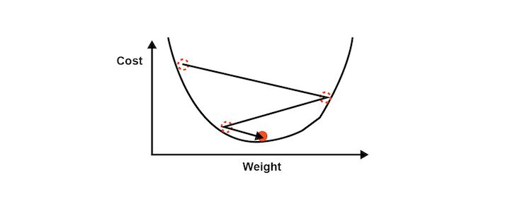
Gradient descent analyses the cost function and it shows via the slope of the curve as shown in the image below. Based on the slope we adjust the weights. This helps to minimise the cost function.

The visualisation of Gradient descent is shown in the diagrams below. The first plot is two dimensional. The image below shows the red circle moving in a zig-zag pattern to reach the minimum cost function eventually.

In the second image, the adjustment of two weights is needed in order to minimise the cost function.

Hence, it can be seen as a contour in the image where the direction is toward the steepest slope and the minimum is to be reached in the shortest time period. This approach does not require a lot of computational processes and the process is not extremely lengthy either. You can say that the training of the model is a feasible task.

Gradient descent can be done in three possible ways,

• Batch gradient descent
• Stochastic gradient descent
• Mini-batch gradient descent

Batch gradient descent

The batch gradient descent is the one in which the cost function is calculated by finding out the sum of all individual cost functions in the training dataset. After this step, the slope is computed by adjusting the weights of the training dataset.

Stochastic gradient descent

In this type of gradient descent, each data entry is followed by the creation of slope of the cost function and the adjustment of the weights in the training dataset. This helps to avoid the local minima if the cost function curve is not convex.

Also, each time the stochastic gradient descent’s process to reach the minimum will appear different.

Mini-batch gradient descent

The third type is the mini-batch gradient descent, which is a combination of batch and stochastic methods. Here, we create different batches by clubbing together multiple data entries in one batch. This essentially results in implementing the stochastic gradient descent on bigger batches of data entries in the training dataset.

While we can dive deep into Gradient Descent, we are afraid it will be outside the scope of the neural network tutorial. Hence let’s move forward and understand how backpropagation works to adjust the weights according to the error which had been generated.

Backpropagation

Backpropagation is an advanced algorithm which enables us to update all the weights in the neural network simultaneously. This drastically reduces the complexity of the process to adjust weights. If we were not using this algorithm, we would have to adjust each weight individually by figuring out what impact that particular weight has on the error in the prediction.

Let us look at the steps involved in training the neural network with Stochastic Gradient Descent:

• Step 1 – Initialise the weights to small numbers. The number should be very close to 0 (but not 0)
• Step 2 – Forward propagation – The neurons are activated from left to right, by using the first data entry in our training dataset, until we arrive at the predicted result y
• Step 3 – Error Computation – Measure the error which will be generated
• Step 4 – Backpropagation – The error generated will be back propagated from right to left. Also, the weights will be adjusted according to the learning rate
• Step 5 – Repeat the previous three steps. The three steps of forward propagation, error computation and backpropagation will go through the entire training dataset
• Step 6 – This would mark the end of the first epoch. The successive epochs will begin with the weight values of the previous epochs, Now, we can stop this process when the cost function reaches an acceptable limit

We have covered a lot in this neural network tutorial and this leads us to apply these concepts in practice. Thus, we will now learn how to develop our own Artificial Neural Network (ANN) to predict the movement of a stock price.

You will understand how to code a strategy using the predictions from a neural network that we will build from scratch. You will also learn how to code the Artificial Neural Network in Python, making use of powerful libraries for building a robust trading model using the power of neural networks.

Stay tuned for the next installment to learn about neural network in trading.

Originally posted on QuantInsti. Visit their blog for additional insights on this topic.