R: Using Differential Evolution to the Nelson-Siegel Model

This post demonstrates the application of Differential Evolution (DE) to estimate Nelson-Siegel parameters using the NMOF R package.

Differential Evolution (DE)

Gilli et al. (2010) applied the Differential Evolution algorithm to the Nelson-Siegel (NS) or Nelson-Siegel-Svensson (NSS) model. The authors implemented and tested this optimization and showed that it is capable of reliably solving the numerical problem of the NS or NSS model.

This DE optimization algorithm can be used from the R package, NMOF, and the authors kindly provided the R code in the appendix of their working paper. This allowed me to apply this code to some data and verify that the estimation results match those obtained using existing algorithms such as the Nelder-Mead.

Following Gilli et al. (2010), there are two notational differences from what I have been accustomed to. First, maturity is expressed in years. Second, the time decay parameter is in reciprocal form, denoted as . Therefore, the NS model is represented as follow.

R code

The following R code estimates the Nelson-Siegel parameters by using the DE.

#========================================================#
# Quantitative Financial Econometrics & Derivatives 
# ML/DL using R, Python, Tensorflow by Sang-Heon Lee 
#
# https://shleeai.blogspot.com
#--------------------------------------------------------#
# Estimating the Nelson-Siegel model 
# using Differential Evolution (DE)
#========================================================#
 
graphics.off(); rm(list = ls())
library(NMOF) # Differential Evolution
    
#-----------------------------------------------
# Objective function
#-----------------------------------------------
    OF <- function(param, data) {
        y <- data$model(param, data$tm)
        maxdiff <- y - data$yM
        
        # max absolute error
        # maxdiff <- max(abs(maxdiff)) 
        
        # Sum of Squares
        maxdiff <- sum(maxdiff^2) 
        
        if (is.na(maxdiff))
            maxdiff <- 1e10
        maxdiff
    }
        
#=======================================================
# 1. Read data
#=======================================================
    
    # b1, b2, b3, lambda, RMSE for comparisons
    ns_reg_para_rmse1 <- c(
        4.26219396, -4.08609206, -4.90893865,  
        3.060792,  0.04883786)
    ns_reg_para_rmse2 <- c(
        4.97628654, -4.75365297, -6.40263059,  
        1.651215,  0.04157326)
    
    str.zero <- "
        mat     rate1      rate2
        3       0.0781     0.0591
        6       0.1192     0.0931
        9       0.1579     0.1270
        12      0.1893     0.1654
        24      0.2669     0.3919
        36      0.3831     0.8192
        48      0.5489     1.3242
        60      0.7371     1.7623
        72      0.9523     2.1495
        84      1.1936     2.4994
        96      1.4275     2.7740
        108     1.6424     2.9798
        120     1.8326     3.1662
        144     2.1715     3.4829
        180     2.5489     3.7827
        240     2.8093     3.9696"
    
    df <- read.table(text = str.zero, header=TRUE)
    m  <- df$mat
    y1 <- df$rate1; y2 <- df$rate2
 
#=======================================================
# 2. Estimation
#=======================================================
    
    #-------------------------------------------------------
    # NS estimation with 1st data
    #-------------------------------------------------------
    data <- list(yM = y1,   # percent
                 tm = m/12, # in years
                 model = NS,
                 ww = 0.1,
                 min = c( 0,-15,-30, 0),
                 max = c(15, 30, 30,10)
                 )
    
    f_penalty <- function(mP, data) {
        minV <- data$min
        maxV <- data$max
        ww <- data$ww
        ## if larger than maxV, element in A is positiv
        A <- mP - as.vector(maxV)
        A <- A + abs(A)
        ## if smaller than minV, element in B is positiv
        B <- as.vector(minV) - mP
        B <- B + abs(B)
        # ## beta 1 + beta2 > 0
        C <- ww*((mP[1L, ] + mP[2L, ]) - abs(mP[1L, ] + mP[2L, ]))
        A <- ww * colSums(A + B) - C
        A
    }
    
    algo <- list(nP = 100L,  ## population size
                 nG = 500L,  ## number of generations
                 F = 0.50,   ## step size
                 CR = 0.99,  ## prob. of crossover
                 min = c( 0,-15,-30, 0),
                 max = c(15, 30, 30,10),
                 pen = f_penalty,
                 repair = NULL,
                 loopOF = TRUE,    ## loop over popuation? yes
                 loopPen = FALSE,   ## loop over popuation? no
                 loopRepair = TRUE, ## loop over popuation? yes
                 printBar = FALSE)
    
    set.seed(90)
    deopt <- DEopt(OF = OF, algo = algo, data = data)
    nsdtim_out1 <- c(deopt$xbest, 
                     sqrt(deopt$OFvalue/length(m)))
    
    #-------------------------------------------------------
    # NS estimation with 2nd data
    #-------------------------------------------------------
    data$yM <- y2
    
    f_penalty <- function(mP, data) {
        minV <- data$min
        maxV <- data$max
        ww <- data$ww
        ## if larger than maxV, element in A is positiv
        A <- mP - as.vector(maxV)
        A <- A + abs(A)
        ## if smaller than minV, element in B is positiv
        B <- as.vector(minV) - mP
        B <- B + abs(B)
       
        # beta 1 + beta2 > 0 is not applied
        
        A <- ww * colSums(A + B) 
        A
    }
    
    # new penalty without beta 1 + beta2 > 0
    algo$pen <- f_penalty
 
    set.seed(90)
    deopt <- DEopt(OF = OF, algo = algo, data = data)
    nsdtim_out2 <- c(deopt$xbest, 
                     sqrt(deopt$OFvalue/length(m)))
    
#=======================================================
# 3. Results and Comparisons
#=======================================================
    
    ns_reg_para_rmse1
    nsdtim_out1
    
    ns_reg_para_rmse2
    nsdtim_out2

As can be seen in the following results, It seems that parameter estimates from the DE algorithm are the same as the benchmark results.

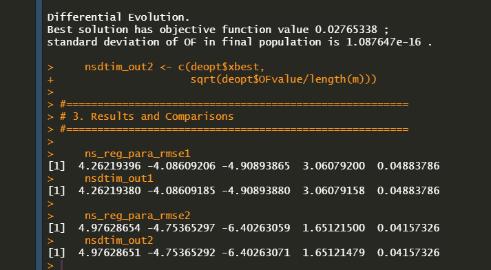
I believe this approach is highly effective in terms of avoiding local minima and achieving fast convergence.

Reference

Gilli, M., S. Große, and E. Schumann (2010). Calibrating the Nelson–Siegel–Svensson model. COMISEF Working Paper Series No. 31.

Originally posted on SHLee AI Financial Model blog.