Understanding Tail Analysis in Financial Markets

The article “Understanding Tail Analysis in Financial Markets” was originally posted on DataGeeek blog.

Source: DataGeeek

In financial markets, distinguishing between information-driven movements and liquidity-driven shocks is critical. The reference study we based our work on highlights the importance of tail analysis: comparing Gaussian (thin-tailed) and Student‑t (fat-tailed) distributions to understand whether price changes are more likely to reflect genuine information or temporary liquidity imbalances.

Financial returns are rarely as well‑behaved as the Gaussian (normal) distribution assumes. In theory, extreme price movements should be exceedingly rare under a thin‑tailed Gaussian model. Yet in practice, markets frequently exhibit fat tails: large jumps, crashes, and spikes that occur far more often than Gaussian theory predicts.

This discrepancy motivates tail analysis—a statistical approach that compares how well different distributions explain the observed data. Two common candidates are:

• Gaussian distribution (thin tails): If returns fit this model better, extreme movements are interpreted as information‑driven. In other words, new information has entered the market, and price changes are more likely to reflect genuine shifts in fundamentals or expectations.
• Student‑t distribution (fat tails): If returns fit this model better, extreme movements are considered liquidity‑driven. These shocks often arise from temporary imbalances in order flow or liquidity constraints, and prices tend to revert once the imbalance subsides.

By comparing the log‑likelihoods of Gaussian and Student‑t fits, we can classify market behavior into these two regimes. This classification is not merely academic: it helps traders, risk managers, and analysts distinguish between trend continuation (information‑driven) and mean reversion (liquidity‑driven).

In our workflow, we apply this tail analysis to gold futures (GC=F) over the past 15 trading days. We compute log returns, fit both distributions, and compare their likelihoods. We then enrich the analysis with a volume impact metric, which highlights whether abnormal trading activity amplifies price changes. Finally, we present the results in a color‑coded audit table that makes tail behavior visually interpretable.

Why These R Packages?

• tidyverse: Provides a consistent grammar for data manipulation (mutate, drop_na, select). It ensures reproducibility and readability when transforming raw market data into log returns and derived metrics.
• tidyquant: Bridges financial data sources with the tidyverse ecosystem. We use it to fetch gold futures data (GC=F) directly from Yahoo Finance, making the workflow self-contained and easy to extend to other tickers.
• MASS: Offers statistical tools for distribution fitting. We rely on fitdistr() to estimate parameters for both Gaussian and Student‑t distributions, enabling a direct comparison of log‑likelihoods.
• gt: Provides professional table rendering. It allows us to format numbers, apply color scales, and highlight audit warnings, turning raw statistical output into a visually interpretable audit table.

library(tidyverse)   # Load tidyverse for data manipulation
library(tidyquant)   # Load tidyquant for financial data retrieval
library(MASS)        # Load MASS for distribution fitting
library(gt)          # Load gt for table rendering
 
ticker <- "GC=F"     # Define the ticker symbol (Gold Futures)
horizon <- 15        # Set horizon to last 15 days
 
# Fetch market data for the chosen ticker and horizon
market_data <- tq_get(ticker, from = Sys.Date() - horizon, to = Sys.Date())
 
# Compute log returns and drop missing values
market_tbl <- market_data %>%
  mutate(returns = log(adjusted) - log(lag(adjusted))) %>%
  drop_na()
 
# Gaussian fit
fit_gauss <- fitdistr(market_tbl$returns, densfun = "normal")
 
# Student-t fit
fit_t <- fitdistr(
  market_tbl$returns,
  densfun = function(x, df, mean, sd) dt((x - mean)/sd, df)/sd,
  start = list(df = 5, mean = mean(market_tbl$returns), sd = sd(market_tbl$returns))
)
 
# Compare log-likelihoods
ll_gauss <- fit_gauss$loglik
ll_t <- fit_t$loglik
signal <- if (ll_gauss > ll_t) "INFO-DRIVEN" else "LIQUIDITY-DRIVEN"
 
# Build audit table
audit_tbl <- market_tbl %>%
  mutate(
    Gaussian_Density = dnorm(returns, mean = mean(returns), sd = sd(returns)),
    StudentT_Density = dt((returns - mean(returns))/sd(returns), df = 5)/sd(returns),
    Volume_Impact = abs(volume)^ifelse(signal == "INFO-DRIVEN", 1.0, 0.6),
    Audit_Warning = signal
  ) %>%
  dplyr::select(Date = date,
                Price = adjusted,
                Gaussian_Density,
                StudentT_Density,
                Volume_Impact,
                Audit_Warning)
 
 
#GT Table
audit_gt <- audit_tbl %>%
  gt() %>%
  tab_header(title = md("**Tail Analysis-Based Audit Table**")) %>%
  cols_label(
    Date = md("**Date**"),
    Price = md("**Price**"),
    Gaussian_Density = md("**Gaussian Density**"),
    StudentT_Density = md("**Student-t Density**"),
    Volume_Impact = md("**Volume Impact**"),
    Audit_Warning = md("**Audit Warning**")
  ) %>%
  fmt_number(columns = c(Price, Gaussian_Density, StudentT_Density, Volume_Impact),
             decimals = 2, use_seps = TRUE) %>%
  data_color(
    columns = c(Price),
    colors = scales::col_numeric(
      palette = c("lightgreen","darkgreen"),
      domain = range(audit_tbl$Price, na.rm = TRUE)
    )
  ) %>%
  data_color(
    columns = c(Gaussian_Density, StudentT_Density),
    colors = scales::col_numeric(
      palette = c("lightblue","darkblue"),
      domain = range(c(audit_tbl$Gaussian_Density,
                       audit_tbl$StudentT_Density), na.rm = TRUE)
    )
  ) %>%
  data_color(
    columns = c(Volume_Impact),
    colors = scales::col_numeric(
      palette = c("pink","red"),
      domain = c(min(audit_tbl$Volume_Impact, na.rm = TRUE),
                 max(audit_tbl$Volume_Impact, na.rm = TRUE))
    )
  ) %>%
  text_transform(
    locations = cells_body(columns = vars(Audit_Warning)),
    fn = function(x) {
      ifelse(x == "INFO-DRIVEN",
             "<span style='color:green;font-weight:bold;'>INFO-DRIVEN</span>",
             "<span style='color:red;font-weight:bold;'>LIQUIDITY-DRIVEN</span>")
    }
  )
 
audit_gt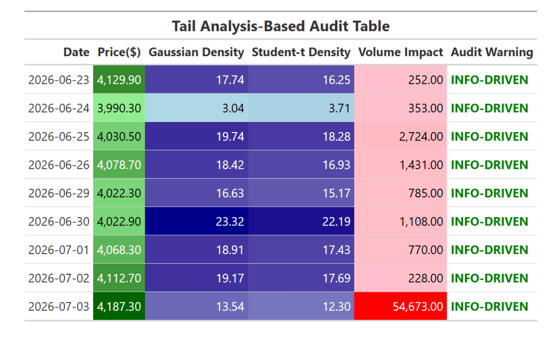

Source: DataGeeek