- Solve real problems with our hands-on interface
- Progress from basic puts and calls to advanced strategies
Interactive Options Course

Posted September 21, 2026 at 12:52 pm

Last updated: September 21, 2026 (originally published October 23, 2024)
Implied shocks are a valuable tool for scenario analysis and are often used to assess the impact of a change in a variable on a portfolio. For example, a change in the yield curve can be used to assess the impact on a fixed-income portfolio; however, the specification of shocks poses challenges and requires an understanding of the methodology as well. In this research paper, we propose an approach to address these challenges by using principal component analysis (PCA) to compute the implied shocks. This paper also presents a methodology to resolve issues related to time-series of eigenanalysis, and applies the specified and PCA implied shocks to a stylized portfolio to compare the approaches. The comparison includes the most negative impact across components, which identifies when the dominant source of variation is not the dominant source of risk for the portfolio. The use of PCA aims to facilitate a more accessible framework for scenario analysis and to deepen the understanding of dynamics driving the scenarios. The numerical calculations, which use online algorithms from the roll package and parallelism from RcppParallel for rolling eigenanalysis of time-series data, are available in the rolleigen package on CRAN: https://cran.r-project.org/package=rolleigen
We illustrate an application of implied shocks in scenario analysis using daily returns for four factors through June 30, 2026: “Equity” (the S&P 500 index, SP500), “Dollar” (the advanced foreign economies U.S. dollar index, DTWEXAFEGS), “Rates” (the 10-year Treasury yield, DGS10), and “Credit” (the high-yield option-adjusted spread, BAMLH0A0HYM2). The methodology depends on the correlation structure of the factors rather than the identity of the factors. The returns are log differences for the return factors and negated level differences for the rate and spread factors, so a positive return is a rally for each factor. The returns are then standardized to unit variance and smoothed as five-day overlapping means to reduce daily noise. The shocks are computed from the standardized returns and then expressed in percent, where each factor’s shock is multiplied by its full-sample standard deviation. The rolling calculations (i.e., the regression betas, the eigenanalysis, and the standard deviations) use a 252-day (one-year) window.
A single factor (or subset of factors) is used to specify shocks, and then shocks are implied across the other factors for the given scenario. Next the specified and implied shocks are applied to assess the impact on a portfolio. Implied shocks are computed using the following methodology:
β = (XT X)-1 XT Y
beta <- solve(crossprod(x)) %*% crossprod(x, y)

implied_shocks <- shocks %*% beta
For example, consider the scenario for specifying the “Equity” factor down one standard deviation:

Data source: Federal Reserve Economic Data (FRED): https://fred.stlouisfed.org/
roll::roll_crossprod(x, y = NULL, width)
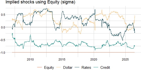
Specifying a single factor (or subset of factors) for computing implied shocks presents challenges. In particular, the specified factor(s) determines both the direction and magnitude of the implied shocks by using the covariance matrix. That is, the direction of the implied shocks is determined by each factor’s correlation with only the specified factor(s). The variance explained by the specified shock also dampens implied shocks on a sigma-adjusted basis by definition. For example, to illustrate the impact of specifying the “Equity” factor on a sigma-adjusted basis, where each factor’s shock is divided by its rolling standard deviation (the returns are standardized to unit variance over the full sample, while the sigma adjustment uses the rolling window):
Data source: Federal Reserve Economic Data (FRED): https://fred.stlouisfed.org/
roll::roll_sd(x, width)
To summarize these challenges, the specified factor(s) determines the direction of the implied shocks and dampens their magnitude on a sigma-adjusted basis. While it is possible to specify all of the shocks to their respective sigmas, the direction of the shocks presents yet another challenge. Using the covariance matrix for guidance is an option, but the selection of the appropriate row and column is subjective. Instead we propose using PCA to identify the direction and magnitude of the shocks that explain the largest share of the variation in the covariance matrix.
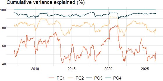
PCA reduces the dimensionality of the data while retaining as much information as possible. Essentially, principal components are computed to capture the maximum variance present in the data. The first principal component explains the most variance, the second principal component (orthogonal to the first) explains the second most, and so on. The proportion of variance explained by the first k principal components is an indicator of the number of components required to reduce the data’s dimension. This calculation is performed using the eigenvalues of the covariance matrix of the standardized returns as follows:

LV <- eigen(cov(x))
L <- LV[["values"]]

variance_explained <- cumsum(L) / sum(L)
Data source: Federal Reserve Economic Data (FRED): https://fred.stlouisfed.org/
rolleigen::roll_eigen(x, width)[["values"]]
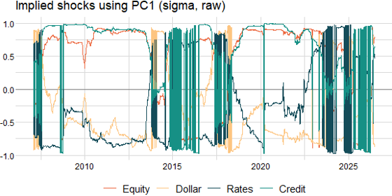
The interquartile range of the variance explained by the first principal component is 50% to 66%. This gives us confidence that the first principal component explains the largest share of the variation in the covariance matrix and can be used to identify the direction and magnitude of the shocks. Specifically, the product of the first eigenvector and square root of the first eigenvalue:

LV <- eigen(cov(x))
L <- LV[["values"]]
V <- LV[["vectors"]]

implied_shocks <- sqrt(L[comp]) * V[ , comp]
Data source: Federal Reserve Economic Data (FRED): https://fred.stlouisfed.org/
rolleigen::roll_eigen(x, width)[["vectors"]]
As illustrated above, we need to resolve issues related to time-series of eigenanalysis: the sign of the eigenvectors can flip and the order of the components can change between windows. These challenges arise given each window is independent of the previous window and floating-point arithmetic is used to calculate the principal components. To address these issues, we can use cosine similarity to match the eigenvectors.
Cosine similarity measures the angle between two vectors in a multidimensional space. The cosine of 0° is 1 and the cosine of 180° is -1; therefore, the cosine similarity between two vectors is 1 if the vectors point in the same direction, -1 if the vectors point in opposite directions, and 0 if the vectors are orthogonal. The cosine similarity between the eigenvectors of the current window and the previous window is calculated as follows:

LV <- eigen(cov(x))
L <- LV[["values"]]
V <- LV[["vectors"]]

cosine_similarity <- crossprod(V, V0) /
  outer(sqrt(colSums(V ^ 2)), sqrt(colSums(V0 ^ 2)))
Note: given the eigenvectors are normalized to unit length, we can ignore the denominator.
The eigenvector with the highest absolute cosine similarity is selected, since a flipped eigenvector scores near -1 rather than 1. The selected eigenvector is multiplied by the sign of the similarity to ensure the eigenvector points in the same direction as the previous window. The eigenvalues are then reordered to match the eigenvectors:
order <- apply(abs(cosine_similarity), 2, which.max)
L <- L[order]
V <- t(sign(diag(cosine_similarity[order, ])) * t(V[ , order]))
Note: the column-by-column match is greedy rather than a strict permutation, so the assignments are not guaranteed to be unique; they are unique in every window of the sample. Hirsa et al. (2023) use an equivalent greedy match and note that tracking additional components before truncation can reduce ordering ambiguity.

Data source: Federal Reserve Economic Data (FRED): https://fred.stlouisfed.org/
rolleigen::roll_eigen(x, width, order = TRUE) # default
Now we have addressed the challenges of specified shocks by using PCA to derive implied shocks. That is, we no longer need to select a single factor (or subset of factors) for computing implied shocks, and PCA selects the direction and magnitude of the shocks that explain the largest share of the variation in the covariance matrix. After the sign is adjusted and eigenvalues are reordered, the implied shocks can be used in time-series analysis as well. As illustrated above, each of the sigma-adjusted implied shocks is less than one in magnitude in every window of the sample. In contrast, the specified approach sets the “Equity” shock to its full standard deviation (i.e., exactly -1 on a sigma-adjusted basis).
The rolling eigenanalysis repeats the decomposition and the cosine similarity ordering for each window, so a naive loop scales with the number of windows. The rolleigen package instead implements the calculation in C++, computes the rolling covariance online via the roll package (i.e., the statistics are updated as observations are added to and removed from a window rather than recomputed from scratch), and uses RcppParallel to parallelize across columns and windows. To compare the approaches, we benchmark a naive loop that matches the ordered output of the roll_eigen function (i.e., an interpreted R loop that computes the eigenanalysis and the cosine similarity ordering for each window) on simulated data at several window widths. The simulation uses 1,000 observations and four variables, matching the number of factors in the application. The roll_eigen function is timed at one thread and at the machine’s default thread count (24 threads) to separate the compiled implementation from the parallelization, and wider cross-sections are also timed at both thread counts to show how the parallelization scales with the cross-section. Both approaches use partial windows (the min_obs argument), so one window ends at each observation and every width computes the same number of windows; the width determines the number of observations within each window instead, which isolates the effect of the width itself:
RcppParallel::setThreadOptions(numThreads = 1) # then the default

result <- microbenchmark::microbenchmark(
  "naive" = naive_eigen(x, width = width, min_obs = min_obs),
  "roll_eigen" = rolleigen::roll_eigen(x, width = width, min_obs = min_obs)
)
| width | naive (ms) | roll_eigen (1 thread, ms) | roll_eigen (24 threads, ms) | speedup vs naive |
| 125 | 503.5 | 4.6 | 4.5 | 109x |
| 250 | 558.0 | 4.9 | 4.5 | 114x |
| 500 | 534.2 | 4.3 | 4.8 | 124x |
Note: the speedup compares the naive loop with the single-thread configuration, so it isolates the compiled implementation and holds the baseline constant across rows.
The median times show that the speedup comes from the compiled implementation, which computes the covariance online, rather than the parallelization at this problem size. The single-thread and default-thread times are roughly equal because each window decomposes a small matrix, so the threading overhead offsets the gains from parallelizing across windows. The naive times are nearly flat across widths because every width computes the same number of windows and the per-window cost is dominated by the interpreted loop overhead rather than by the number of observations within each window. The roll_eigen times are also consistent across widths, though for a different reason: the online covariance updates make the per-window cost independent of the width.
| n_vars | roll_eigen (1 thread, ms) | roll_eigen (24 threads, ms) | speedup vs 1 thread |
| 10 | 18.4 | 8.1 | 2.3x |
| 25 | 124.0 | 34.4 | 3.6x |
| 50 | 759.2 | 269.4 | 2.8x |
Note: the wider cross-sections use a width of 250; the speedup compares one thread with the machine’s default thread count, so it isolates the parallelization; at four variables the single-thread and default-thread times are roughly equal, as shown in the previous table.
The parallelization is additive at wider cross-sections, but the gain does not scale monotonically: the speedup over one thread peaks at roughly 3.6x in the tens of variables and partly declines at 50 variables. The gain also remains well below the thread count because each window’s decomposition is small relative to the synchronization cost. Overall the roll_eigen function is roughly two orders of magnitude faster than the naive loop at four variables (i.e., the four factors in the application), which makes the time-series of eigenanalysis practical for scenario analysis at daily frequencies.
Next we apply the specified and PCA implied shocks to a stylized portfolio to compare the approaches. The portfolio allocates 60% to the “Equity” factor and 40% to a proxy for an aggregate bond index, analogous to a generic 60/40 stock/bond allocation. The proxy applies a duration of 6 to the “Rates” factor and a spread exposure of 0.6 to the “Credit” factor. The estimated impact for each scenario is the product of the portfolio exposures and the shocks:

where e is the vector of portfolio exposures, σ is the vector of full-sample standard deviations, and s is the vector of specified and implied shocks for the scenario computed from the standardized returns. The specified scenario shocks the “Equity” factor down one standard deviation, the adverse direction for scenario analysis, and implies the shocks across the other factors. The PCA scenario uses the first principal component oriented so the “Equity” element is negative, matching the adverse direction of the specified scenario. Both scenarios are annualized (the scaling reflects both the daily frequency and the five-day overlap) and expressed in percent.
We also extend the comparison to every principal component by orienting each component against the portfolio. That is, the most negative impact of a one standard deviation move in each component, annualized and expressed in percent on the same basis as the specified and PCA scenarios:

LV <- eigen(cov(x))
L <- LV[["values"]]
V <- LV[["vectors"]]

impacts <- -abs(sqrt(L) * crossprod(V, exposures * sd_full))
The most negative impact across components is the worst single-component scenario and does not depend on the sign of the eigenvectors, while the component labels follow the cosine similarity ordering. The one standard deviation portfolio loss bounds both the specified scenario and the most negative impact. The specified scenario equals that loss scaled by the correlation between the portfolio and the specified factor because the specified shock is one standard deviation and the implied shocks are regression betas on that factor. The sum of squared impacts equals the portfolio variance, so the most negative impact cannot exceed that loss. Note that the minimum across components is a selected worst case rather than a probability-consistent scenario because each impact is a one standard deviation move of a different component.
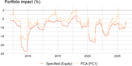
After the shocks are computed, we compare the estimated impact for each scenario over time. The chart below shows the estimated impact of the specified and PCA scenarios for the stylized portfolio.
Data source: Federal Reserve Economic Data (FRED): https://fred.stlouisfed.org/
The two scenarios produce similar estimated impacts over most of the sample: the average is roughly -10% for the specified scenario and -7% for the PCA scenario, and the correlation between the two series is 0.93. The specified scenario is larger in magnitude on average because it sets the “Equity” shock to its full standard deviation. The first principal component explains roughly half to two-thirds of the variation in the covariance matrix, which dampens each factor’s shock on a sigma-adjusted basis by definition. The scenarios diverge when the composition of the first principal component changes: the difference peaks at roughly 12 percentage points in December 2009, when the “Equity” element of the first principal component shrinks toward zero, as illustrated in the implied shocks using PC1 above. The estimated PCA impact for the stylized portfolio therefore rises toward zero while the specified scenario, which sets “Equity” to its full standard deviation, remains large in magnitude. The comparison attributes the difference in estimated impact to the construction of the scenarios, specifically the choice of specified versus PCA implied shocks, rather than to the factors themselves.
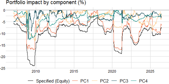
The chart below extends the comparison to the most negative impact for each component, together with the specified scenario.
Data source: Federal Reserve Economic Data (FRED): https://fred.stlouisfed.org/
The most negative impact across components averages roughly -8%, between the PCA and specified scenarios, and its correlation with the specified scenario is 0.96, higher than for the first principal component alone. On average the most negative component accounts for 78% of the one standard deviation portfolio loss, which also averages roughly -10%, the same as the specified scenario. The correlation between the portfolio and the “Equity” factor averages roughly 0.98 because the “Equity” allocation dominates portfolio volatility. The component with the most negative impact also rotates over time: in December 2009, the impact of the first principal component is roughly -5% while the impact of the second principal component is roughly -12%. The first principal component carries roughly 10% of the variation in the “Equity” factor at that date while the second principal component carries roughly 51% of it. The most negative impact therefore remains closer to the specified scenario, which shocks the “Equity” factor directly, than the first principal component alone does. That is, the most negative component identifies when the dominant source of variation is not the dominant source of risk for the portfolio.
This research paper introduced an approach to implied shocks that used PCA to address challenges associated with specified shocks. The methodology not only offered a more accessible framework for scenario analysis but also enhanced the understanding of dynamics driving the scenarios. By using PCA to derive implied shocks and resolving issues related to time-series of eigenanalysis, the methodology both simplified and improved the construction of scenarios. The benchmark showed the compiled and parallelized implementation in the rolleigen package is roughly two orders of magnitude faster than a naive loop. The application to a stylized portfolio illustrated how the choice of scenario construction affects the estimated impact, including the most negative impact across components as a portfolio-oriented scenario. The methodology presented can provide valuable insights for risk managers seeking to refine implied shocks and make more informed decisions on scenario analysis. The rolleigen package is available for R; for more on the underlying eigenanalysis, go to https://jasonjfoster.github.io/posts/eigen-r/ for R code and https://jasonjfoster.github.io/posts/eigen-py/ for Python code.
rolleigen is a package that provides fast and efficient computation of rolling and expanding eigenanalysis for time-series data.
install.packages("rolleigen")# install.packages("pak")
pak::pak("jasonjfoster/rolleigen") # roll (>= 1.1.7)library(rolleigen)
The rolleigen::roll_eigen function computes the rolling and expanding eigenvalues and eigenvectors of time-series data.
Parameters
Value
A list that contains values, an object of the same class and dimension as x with the rolling and expanding eigenvalues, and vectors, a cube with each slice the rolling and expanding eigenvectors.
Examples
n <- 15
m <- 3
x <- matrix(rnorm(n * m), nrow = n, ncol = m)
weights <- 0.9 ^ (n:1)

# rolling eigenvalues and eigenvectors with complete windows
rolleigen::roll_eigen(x, width = 5)

# rolling eigenvalues and eigenvectors with partial windows
rolleigen::roll_eigen(x, width = 5, min_obs = 1)

# expanding eigenvalues and eigenvectors with partial windows
rolleigen::roll_eigen(x, width = n, min_obs = 1)

# expanding eigenvalues and eigenvectors with partial windows and weights
rolleigen::roll_eigen(x, width = n, min_obs = 1, weights = weights)
Hirsa, A., Klinkert, F., Malhotra, S., & Holmes, R. (2023). “Robust Rolling PCA: Managing Time Series and Multiple Dimensions.” SSRN. https://ssrn.com/abstract=4400158.
Zoonekynd, V. (2012). “Time series of PCA – Sign change in factor loadings [Answer].” Quantitative Finance Stack Exchange. https://quant.stackexchange.com/a/3095.
Information posted on IBKR Campus that is provided by third-parties does NOT constitute a recommendation that you should contract for the services of that third party. Third-party participants who contribute to IBKR Campus are independent of Interactive Brokers and Interactive Brokers does not make any representations or warranties concerning the services offered, their past or future performance, or the accuracy of the information provided by the third party. Past performance is no guarantee of future results.
This material is from Jason Foster and is being posted with its permission. The views expressed in this material are solely those of the author and/or Jason Foster and Interactive Brokers is not endorsing or recommending any investment or trading discussed in the material. This material is not and should not be construed as an offer to buy or sell any security. It should not be construed as research or investment advice or a recommendation to buy, sell or hold any security or commodity. This material does not and is not intended to take into account the particular financial conditions, investment objectives or requirements of individual customers. Before acting on this material, you should consider whether it is suitable for your particular circumstances and, as necessary, seek professional advice.
The third-party code discussed within this article is not investment or trading advice, and is for proof-of-concept, educational, and illustrative purposes only. IBKR makes no representations or warranty regarding its accuracy or completeness. Users are solely responsible for conducting their own independent testing and due diligence before applying any code or concepts in a live or production environment
Please keep in mind that the examples discussed in this material are purely for technical demonstration purposes, and do not constitute trading advice. Also, it is important to remember that placing trades in a paper account is recommended before any live trading.
There is a substantial risk of loss in foreign exchange trading. The settlement date of foreign exchange trades can vary due to time zone differences and bank holidays. When trading across foreign exchange markets, this may necessitate borrowing funds to settle foreign exchange trades. The interest rate on borrowed funds must be considered when computing the cost of trades across multiple markets.











Join The Conversation
For specific platform feedback and suggestions, please submit it directly to our team using these instructions.
If you have an account-specific question or concern, please reach out to Client Services.
We encourage you to look through our FAQs before posting. Your question may already be covered!