Ito’s Lemma Applied to Stock Trading

The article “Ito’s Lemma Applied to Stock Trading” first appeared on QuantInsti blog.

This is the second part of the two-part blog where we explore how Ito’s Lemma extends traditional calculus to model the randomness in financial markets. Using real-world examples and Python code, we’ll break down concepts like drift, volatility, and geometric Brownian motion, showing how they help us understand and model financial data, and we’ll also have a sneak peek into how to use the same for trading in the markets.

In the first part, we saw how classical calculus cannot be used for modeling stock prices, and in this part, we’ll have an intuition of Ito’s lemma and see how it can be used in the financial markets. Here’s the link to part I, in case you haven’t gone through it yet: https://blog.quantinsti.com/itos-lemma-trading-concepts-guide/

This blog covers:

• Pre-requisites
• Quick Recap
• Ito Calculus
• Ito’s Lemma Applied to Stock Prices
• Use Case – I of Ito’s Lemma
• Important Considerations
• Use Case – II of Ito’s Lemma
• Till Next Time

Pre-requisites

You will be able to follow the article smoothly if you have elementary-level proficiency in:

• Calculus
• Python coding

Quick Recap

In part I of this two-blog series, we learned the following topics:

1. The chain rule
2. Deterministic and stochastic processes
3. Drift and volatility components of stock prices
4. Weiner processes

In this part, we shall learn about Ito calculus and how it can be applied to the markets for trading.

Ito Calculus

Remember  from part I?  is why Ito came up with the calculus he did. In classical calculus, we work with functions. However, in finance, we frequently work with stochastic processes, where  represents stochasticity.

Rewriting the equations from part I:

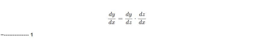
The equation for chain rule:

The equation for geometric Brownian motion (GBM):

Equation 2 is a differential equation. The presence of  makes the GBM a stochastic differential equation (SDE).  What’s so special about SDEs?

Remember the chain rule discussed in part I? That’s only for deterministic variables. For SDEs, our chain rule is Ito’s lemma!

Let’s get down to business now.

Ito’s Lemma Applied to Stock Prices

The following equation is an expression of Ito’s lemma:

Here,

f(x) is a function which can be differentiated twice, and

S is a continuous process, having bounded variation

What do we mean by bounded variation?

It simply means that the difference between St+1 and St, for any value of t, would never exceed a certain value. What this ‘certain value’ is, is not of much significance. What is significant is that the difference between two consecutive values of the process is finite.

Next question:

What’s 

It’s a notation.

Of what?

A notation to denote a quadratic variation process.

What’s that?

In this blog, we won’t get into the intuition of the quadratic variation. It would suffice to know that the quadratic variation of 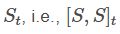is as follows:

If St follows a Brownian motion, the derivative of its quadratic variation is:

Substituting equation 4 in equation 3, we get:

How is this derived?

We can treat equation 5 as a Taylor series expansion till the second order. If you aren’t familiar with it, don’t worry; you can continue reading.

Still, what’s the intuition? Here, f is a function of the process S, which itself is a function of time t. The change in f depends on:

1. The first-order partial derivative of f with respect to S,
2. The second-order partial derivative of f with respect to t,
3. The square of the volatility σ, and,
4. The square of S.

The last three are multiplied and then added to the first one.

We saw earlier that stock returns follow a Brownian motion, so stock prices follow a GBM. Hence,  suppose we have a process Rt, which is equal to

If we take in the GBM SDE (equation 2), and if we use the expression for Ito’s lemma (equation 3), we’ll have:

and,

Since

and

(equation 4),

we can rewrite equation 7 as:

Since the second term on the RHS doesn’t depend on the LHS, we can use direct integration to solve equation 7:

Since

Thus, equation 9 changes to:

Let’s understand what the equation means here. The stock price at time t = 0, when multiplied by this term:

would give the stock price at time t.

In equation 2, the drift component had just μ, but in equation 10, we subtract σ2/2 from μ. Why so? Remember how we obtain μ? By taking the mean of daily log returns, right?

Umm, no! As mentioned in part I, μ is the average percentage drift (or returns), and NOT the logarithmic drift.

As we saw from the drift component and volatility component graphs, the close price isn’t just the drift component, but also the volatility component added to it. Hence, we need to correct the drift to consider the volatility component as well. It is towards this correction that we subtract from μ. The intuition here is that the arithmetic mean of a set of non-negative real numbers is greater than or equal to the geometric mean of the same set of numbers. The value of μ before the correction is the arithmetic mean, and after the correction, it is close to the geometric mean. When taken on an annual basis, the geometric mean is the CAGR.

How do we interpret equation 10? The current stock price is simply a function of the past stock price, the corrected drift, and the volatility.

How do we use this in the markets? Let’s see…

Use Case – I of Ito’s Lemma

Note: The codes in this part are continued from part I, and the graphs and values obtained are as of October 18, 2024.

# Calculating the daily percent returns
msft["Daily_Returns"] = msft["Close"].pct_change()

# Calculating mean, standard deviation, and variance of daily percent returns
daily_mean = msft["Daily_Returns"].mean()
daily_stdev = msft["Daily_Returns"].std()
daily_var = daily_stdev**2
print("The mean of the daily percent returns = " + str(np.round(daily_mean,5)))
print("The standard deviation of the daily percent returns = " + str(np.round(daily_stdev,5)))
print("The variance of the daily percent returns = " + str(np.round(daily_var,5)))

Daily_percent_returns.py hosted with ❤ by GitHub

Output:

The mean of the daily percent returns = 0.00109
The standard deviation of the daily percent returns = 0.01707
The variance of the daily percent returns = 0.00029

# Calculating the daily compounded returns
daily_compounded_mean = (((msft["Close"][-1]/msft["Close"][0])**(1/len(msft)))-1)
print("Daily compounded returns = " + str(np.round(daily_compounded_mean,8)))

Daily_compound_returns.py hosted with ❤ by GitHub

Output:

Daily compounded returns = 0.00094878

# Calculating the correct daily percent returns
corrected_mean = (daily_mean - (daily_stdev**2)/2)
print("Corrected daily percent returns = " + str(np.round(corrected_mean,8)))

Correct_daily_percent_returns hosted with ❤ by GitHub

Output:

Corrected daily percent returns = 0.000949

The arithmetic mean of the returns was initially 0.00109, and the geometric mean (daily compounded returns) computes to 0.00094878. After incorporating the drift correction, the arithmetic mean stood at 0.000949. Quite close to the geometric mean!

How do we use this for trading?

Suppose we wanna predict the range within which the price of Microsoft is likely to lie after, say, 42 trading days (2 calendar months) from now.

Let’s seek refuge in Python again:

# Calculating the convexity corrected drift (mean), variance, and standard deviation for 42 trading days
mean_42 = (daily_mean - (daily_stdev**2)/2 ) * 42
var_42 = daily_var * 42
stdev_42 = np.sqrt(var_42)
print("Corrected drift for 42 days = " + str(np.round(mean_42,8)))
print("Variance for 42 days = " + str(np.round(var_42,8)))
print("Standard deviation for 42 days = " + str(np.round(stdev_42,8)))

Convexing_corrected_drift.py hosted with ❤ by GitHub

Output:

Corrected drift for 42 days = 0.03985788
Variance for 42 days = 0.01223456
Standard deviation for 42 days = 0.11060996

# Calculating the likely returns of Microsoft after 42 trading days

# Lower and upper ranges of Microsoft returns after 42 days, with 95% likelihood
lower_return_42 = mean_42 - 2 * stdev_42
upper_return_42 = mean_42 + 2 * stdev_42

# Lower and upper ranges of Microsoft prices after 42 days, with 95% likelihood
lower_price_42 = msft["Close"][-1] * np.exp(lower_return_42)
upper_price_42 = msft["Close"][-1] * np.exp(upper_return_42)

print("Price below which the stock isn't likely to trade with a 95% probability after 42 days = " + str(np.round(lower_price_42,2)))
print("Price above which the stock isn't likely to trade with a 95% probability after 42 days = " + str(np.round(upper_price_42,2)))

Likely_return_Microsoft.py hosted with ❤ by GitHub

Output:

Price below which the stock isn’t likely to trade with a 95% probability after 42 days = 347.6
Price above which the stock isn’t likely to trade with a 95% probability after 42 days = 541.04

We know with 95% confidence between which ranges the stock is likely to lie after 42 trading days from now! How do we trade this? Ways are many, but I’ll share one specific method.

# Downloading the option chain of Microsoft with expiry on the 20th of December 2024, two months from now
msft_optc = yf.Ticker("MSFT").option_chain('2024-12-20')

# Selecting the put with a strike of $345, and the call with strike of $545

put_345 = msft_optc.puts[msft_optc.puts['strike'] == 345]
call_545 = msft_optc.calls[msft_optc.calls['strike'] == 545]

print("Put with strike 345:\n", put_345)
print("\nCall with strike 545:\n", call_545)

Download_and_print.py hosted with ❤ by GitHub

Output:

Put with strike 345:
          contractSymbol             lastTradeDate  strike  lastPrice  bid  \
44  MSFT241220P00345000 2024-10-17 19:44:37+00:00   345.0       1.53  0.0   

    ask  change  percentChange  volume  openInterest  impliedVolatility  \
44  0.0     0.0            0.0     1.0             0           0.125009   

    inTheMoney contractSize currency  
44       False      REGULAR      USD  

Call with strike 545:
          contractSymbol             lastTradeDate  strike  lastPrice  bid  \
84  MSFT241220C00545000 2024-10-16 13:45:27+00:00   545.0       0.25  0.0   

    ask  change  percentChange  volume  openInterest  impliedVolatility  \
84  0.0     0.0            0.0     169             0           0.125009   

    inTheMoney contractSize currency  
84       False      REGULAR      USD 

We have chosen out-of-the-money strikes near the 95% confidence price range we obtained earlier.

This way, we can pocket around $1.53 + $0.25 (emboldened in the above output) = $1.78 per pair of stock options sold, if held till expiry. If we sell one lot each of these call and put option contracts, we can pocket $178, since the lot size is 100. And what’s the assurance of us making this profit? 95%, right? Simplistically, yes, but let’s move closer to reality now.

Important Considerations

Assumption of Normality: We used mean +/- 2 standard deviations and kept talking about 95% confidence. This works in a world where the stock returns are normally distributed. But in the real world, they are not! And more often than not, this deviation from a normal distribution works against us since people react faster to news of impending doom over news of euphoria.

Transaction Costs: We didn’t consider the transaction costs, taxes, and implementation shortfalls.

Backtesting: We haven’t backtested (and forward tested) whether the prices have historically lied (and would lie in the future) within the predicted price ranges.

Opportunity Costs: We also didn’t consider the margin requirements and the opportunity costs, were we to deploy some margin amount in this strategy.

Volatility: Finally, we are trading volatility here, not the price. We’ll end up pocketing the whole premium only if both the options expire worthless, i.e., out-of-the-money. But for that to happen, the volatility must be low until the expiry. We must account for the implied volatilities obtained in the previous code output. Oh, and by the way, how is this implied volatility calculated?

Use Case – II of Ito’s Lemma

We calculate the implied volatility from the classic Black-ScholesMerton model for option pricing. And how did Fischer Black, Myron Scholes, and Robert Merton develop this model? They stood on the shoulders of Kiyoshi Ito!

Till Next Time

And this is where I bid au revoir! Do backtest the code and check whether it can predict the range of future prices with reasonable accuracy. You can also use mean +/- 1 standard deviation in place of 2 standard deviation. The benefit? The range would be tighter, and you could pocket more premium. The flip side? The chances of being profitable get reduced to around 68%! You can also think of other ways how to capitalise on this prediction. Do let us know in the comments what you tried.

References:
Main Reference:
https://research.tilburguniversity.edu/files/51558907/INTRODUCTION_TO_FINANCIAL_DERIVATIVES.pdf
Auxiliary References:
Wikipedia pages of Ito’s lemma, Brownian motion, geometric Brownian motion, quadratic variation, and, AM-GM inequality
EPAT lectures on statistics and options trading