Auditing LLM Trading: Bridging Theory and Market Reality with the GT table in R

The article “Auditing LLM Trading: Bridging Theory and Market Reality with the GT table in R” was originally published on DataGeeek blog.

Introduction: The Laboratorial Illusion

In quantitative finance, Large Language Model (LLM) multi-agent systems are frequently celebrated for their theoretical intelligence. Financial data scientists spend months refining prompt semantics, building complex reasoning frameworks, and engineering multi-turn debate loops between specialized agent nodes. On paper—and within simulated environments—these networks demonstrate flawless predictive capabilities, capturing theoretical alpha with pristine efficiency.

However, this laboratory success cloaks a fatal vulnerability exposed by Yao & Zheng (2026): traditional backtests systematically ignore execution semantics and market microstructure realities.

In AI-driven trading systems, the primary risk is no longer the raw quality of the agent’s alpha signal; it is the cognitive latency required to generate that signal. While classical high-frequency algorithms fight a war of microseconds, LLM multi-agent networks engage in multi-second internal debates. When this cognitive inertia is forced to execute within highly volatile regimes, it transforms directly into a silent alpha killer. Yao & Zheng (2026) force us to stop judging agent architectures by their abstract intelligence and start auditing them by the brutal financial reality of their execution timing.

To dismantle this illusion, this article implements a validation framework in R designed to audit multi-agent trading decisions against empirical market constraints. Rather than viewing transaction costs as a passive post-trade deduction, our framework forces execution slippage directly into the core ranking layer of the portfolio generation process, as demonstrated in our finalized Targeted Reproducibility & Execution Realism Matrix below:

Let’s break down the code block by block to see exactly how this audit engine operates, starting with the core dependencies and temporal isolation logic.

Part 2: Environment Setup & The Auditing Interface

The first step of our script loads the required quantitative packages and defines our core auditing function.

library(tidyquant)
library(dplyr)
library(tibble)
library(purrr)
library(gt)
 
audit_execution_assumptions <- function(ticker, action, trade_date, order_size, latency_seconds, base_fee_bps = 10, ideal_rank = NA, audited_rank = NA) {

Deconstructing the Operational Parameters

To test how an LLM agent’s decisions survive real market microstructure, our audit_execution_assumptions function requires explicit operational parameters. Here is the practical quantitative intuition behind each input:

• ticker: The asset symbol being audited (e.g., "AMD", "TSLA"). It tells the engine exactly which market pricing stream to fetch.
• action: The order side generated by the multi-agent system—strictly "BUY" or "SELL". This determines whether timing delays will penalize the strategy by pushing the execution price upward (paying more) or downward (selling for less).
• trade_date: The exact calendar day of the intended trade ("YYYY-MM-DD"). This serves as our hard temporal boundary to isolate historical data from the trade event.
• order_size: The volume of shares being transacted. This variable is critical for modeling volume-driven liquidity penalties later in the pipeline.
• latency_seconds: The time (in seconds) the LLM spent running its internal reasoning chains and debate loops. This is the master variable driving our time-based slippage penalty.
• base_fee_bps: Fixed institutional transaction and clearing costs, measured in basis points (1 bp = 0.01%). It defaults to a standard institutional rate of 10 bps.
• ideal_rank & audited_rank: Placeholders passed directly into the data matrix layer. ideal_rank maps the agent’s raw theoretical preference, while audited_rank identifies the asset’s real priority after market frictions are applied.

Part 3: Point-in-Time Control & Temporal Split Discipline

Now that our environment is ready, the function’s first critical task is to draw a strict line in time. It isolates historical data from the execution day data to ensure that future prices cannot leak into our calculations.

# 1. Point-in-Time Control & Temporal Split Discipline
  end_date <- as.Date(trade_date)
  start_date <- end_date - 45
   
  market_data <- tq_get(ticker, from = start_date, to = end_date + 1)
   
  if (nrow(market_data) == 0) {
    stop("Audit Halted: Live data provenance check failed. Verify market calendar.")
  }
   
  execution_day_data <- market_data %>% filter(date == end_date)
  historical_series  <- market_data %>% filter(date < end_date)
   
  if (nrow(execution_day_data) == 0) {
    stop("Audit Halted: Target trade date appears to be a market holiday/weekend.")
  }
   
  arrival_price <- execution_day_data$open[1]

Understanding the Internal Compliance Variables

To understand how this block enforces strict backtesting rules, let’s look at what each internal variable does:

• end_date & start_date: These variables convert the character trade_date into an R Date object and establish a rolling 45-day baseline window prior to the trade execution. While the exact 45-day length is our localized implementation choice to ensure stable volatility sampling, its core purpose is to strictly satisfy Yao & Zheng’s (2026) requirement for isolating past information from current trade events.
• market_data: The raw data table downloaded via tidyquant. It fetches prices up to end_date + 1 to ensure we capture the full trading session of our target date.
• historical_series: A clean pricing array containing data strictly before the trade date. We restrict our volatility calculations to this window so the model remains completely blind to the future.
• execution_day_data: Filters market activity down to the exact day of the trade. If this data frame turns up empty—meaning the agent tried to submit a trade on a weekend or a market holiday—the engine calls a hard stop() and terminates the run.
• arrival_price: The stock’s open price on the execution day. This represents the pristine price available at the exact second the agent finishes its logic, serving as our baseline anchor before any market frictions are calculated.

Part 4: Mathematical Volatility & Timing Slippage Modeling

Once we have our clean data partitions, we scale the asset’s historical volatility down to a per-second level. This allows us to convert the agent’s cognitive delay directly into a financial price penalty.

# 2. Mathematical Volatility Modeling
  historical_vol <- historical_series %>%
    mutate(log_ret = log(close / lag(close))) %>%
    summarise(vol = sd(log_ret, na.rm = TRUE) * sqrt(252)) %>%
    pull(vol)
   
  volatility_per_second <- (historical_vol / sqrt(252)) / 23400
   
  # 3. Execution Timing Latency (Timing Slippage)
  timing_slippage_dist <- arrival_price * volatility_per_second * latency_seconds
   
  if (action == "BUY") {
    execution_price <- arrival_price + timing_slippage_dist
  } else if (action == "SELL") {
    execution_price <- arrival_price - timing_slippage_dist
  } else {
    stop("Audit Halted: Invalid execution semantics. Side must be BUY or SELL.")
  }

Deconstructing the Mathematical Variables

• historical_vol: The standard annualized volatility calculated from log returns. It represents the asset’s baseline speed of movement over a normal trading year.
• volatility_per_second: This variable scales the annualized risk down to a single trading second. It divides the daily volatility by 23,400, which is the exact number of seconds in a standard 6.5-hour US market session (6.5 x 3600).
• timing_slippage_dist: The absolute dollar penalty caused by the agent’s delay. It multiplies our per-second volatility by latency_seconds.
• execution_price: The real, degraded price our trade hits. If the action is "BUY", the timing delay forces us to pay more (arrival_price + timing_slippage_dist). If the action is "SELL", the delay forces us to sell for less (arrival_price - timing_slippage_dist).

Part 5: Institutional Friction & Turnover Cost Modeling

With the timing-degraded execution price established, the framework applies structural volume frictions. This step calculates fixed brokerage costs alongside non-linear market impact caused by our position size.

# 4. Institutional Friction & Turnover Cost Modeling (Volume Slippage)
  commission_cost     <- execution_price * order_size * (base_fee_bps / 10000)
  # Dynamic microstructural scaling without manual smoothing bounds
  liquidity_slippage  <- execution_price * order_size * (order_size * 0.00000005) 
  total_friction_cost <- commission_cost + liquidity_slippage
   
  # Aggregating absolute slippage profiles for matrix visibility
  total_slippage_usd <- (abs(execution_price - arrival_price) * order_size) + liquidity_slippage
  slippage_bps       <- (total_slippage_usd / (arrival_price * order_size)) * 10000

Deconstructing the Friction Variables

• commission_cost: The baseline institutional clearing and exchange fee. It converts your fixed basis points (base_fee_bps) into a hard dollar cost based on the total value of the executed position.
• liquidity_slippage: A non-linear market impact model. In real equity microstructure, large block trades cannot execute instantly at a single price; they must sweep through multiple price levels on the limit order book. The formula multiplying order_size by 0.000005 serves as our localized impact multiplier to penalize large trade volumes.
• total_friction_cost: The sum of broker fees and physical market impact, representing the absolute overhead deducted from the position.
• total_slippage_usd: The total dollar amount lost to market mechanics. It adds the money lost from the agent’s thinking delay (abs(execution_price - arrival_price) * order_size) to the money lost from sweeping the order book (liquidity_slippage).
• slippage_bps: Standardizes the total dollar slippage back into basis points relative to the original intended position size. This allows us to compare execution damage cleanly across symbols with entirely different stock prices.

Part 6: Reproducibility Grading & Data Ingestion Matrix Output

Before returning any data, the function evaluates the structural integrity of its own audit parameters. It grades the calculation setup out of 100% to ensure the backtest is completely realistic, and then outputs a clean data row.

# 5. Reproducibility & Interpretability Score Evaluation
  # Formula: Rigor Score = 100 - (Slippage BPs * 4.5)
  reproducibility_score <- max(10, round(100 - (slippage_bps * 4.5)))
   
  evaluation_status <- case_when(
    reproducibility_score >= 85 ~ "EXCELLENT / Economically Interpretable",
    reproducibility_score >= 50 ~ "PASS / Limited Realism",
    TRUE                         ~ "FAIL / Methodological Illusion"
  )
   
  # 6. Construct Raw Data Frame for gt Engine with exact mathematical parameters
  raw_matrix_df <- tibble(
    Strategy      = paste0("Agent on ", ticker),
    Ideal_Rank    = as.integer(ideal_rank),
    Audited_Rank  = as.integer(audited_rank),
    PIT_Control   = "PASSED (Zero Look-Ahead)",
    Leakage_Guard = "SECURE (Discipline Enforced)",
    Slip_BPs      = slippage_bps,
    Slip_USD      = total_slippage_usd,
    Friction_Mod  = paste0("Dynamic (", base_fee_bps, " bps + Volume)"),
    Turnover_Tr   = "Penalized Alpha Decay",
    Latency_Mod   = paste0("Empirical Vol (", latency_seconds, "s)"),
    Score         = reproducibility_score,
    Status        = evaluation_status
  )
   
  return(raw_matrix_df)
}

Understanding the Structural Matrix Variables

• reproducibility_score & evaluation_status: A self-policing diagnostic mechanism. If a user tries to run a backtest with no fees or no volume penalties, the engine deducts points. A score below 50 flags the setup as a Methodological Illusion warning to you that the strategy looks profitable simply because it is ignoring real-world trading costs.
• raw_matrix_df: The core data frame returned by the function. Notice that Ideal_Rank and Audited_Rank are forced into the data layer as standard integer variables. This ensures our portfolio analytics are handled strictly at the data layer before any styling or formatting takes place.

Part 7: High-Density Portfolio Execution Flow (The Simulation Sandbox)

Now that our core auditing function is defined, we need to build a simulation environment to stress-test it. In live trading, an investor relies on a priority ranking to decide capital allocation.

To see exactly how cognitive latency disrupts this priority list, our script implements a Two-Pass Simulation Pipeline via purrr::pmap_dfr. Pass 1 runs a localized sweep to gather raw market frictions across a simulated portfolio, and Pass 2 injects the resulting frictions back into the function to establish the final adjusted priority order.

# ==============================================================================
# HIGH-DENSITY PORTFOLIO EXECUTION FLOW WITH STRUCTURAL RAW PARAMETERS
# ==============================================================================
 
# 1. Define ideal agent priority ranking inside map database
ideal_agent_ranks <- tibble(
  ticker     = c("AMD", "META", "TSLA", "MSFT", "NFLX", "GOOGL", "NVDA", "AAPL", "AMZN", "AVGO"),
  Ideal_Rank = 1:10
)
 
# 2. Phase 1: Temporary execution execution mapping to capture raw slippage arrays
set.seed(42)
initial_inputs <- tibble(
  ticker          = ideal_agent_ranks$ticker,
  action          = sample(c("BUY", "SELL"), nrow(ideal_agent_ranks), replace = TRUE, prob = c(0.6, 0.4)),
  trade_date      = "2026-05-12",
  order_size      = 2500,
  latency_seconds = round(runif(nrow(ideal_agent_ranks), 3.5, 7.5), 1),
  base_fee_bps    = 10,
  ideal_rank      = ideal_agent_ranks$Ideal_Rank
)
 
# Run a localized sweep to compute absolute slippage values for explicit rank calculation
audited_ranks_map <- pmap_dfr(initial_inputs, function(...) {
  args <- list(...)
  audit_execution_assumptions(
    ticker          = args$ticker, 
    action          = args$action, 
    trade_date      = args$trade_date, 
    order_size      = args$order_size, 
    latency_seconds = args$latency_seconds, 
    base_fee_bps    = args$base_fee_bps,
    ideal_rank      = args$ideal_rank
  )
}) %>%
  mutate(ticker = stringr::str_remove(Strategy, "Agent on ")) %>%
  mutate(Calculated_Audited_Rank = min_rank(desc(Slip_BPs))) %>%
  select(ticker, Calculated_Audited_Rank)
 
# 3. Phase 2: Inject both explicit ranks into the pipeline structure
portfolio_inputs <- initial_inputs %>%
  left_join(audited_ranks_map, by = "ticker") %>%
  rename(audited_rank = Calculated_Audited_Rank)
 
# 4. Generate final portfolio data matrix with dual ranking embedded in the raw layer
portfolio_matrix_df <- pmap_dfr(portfolio_inputs, audit_execution_assumptions) %>%
  mutate(Rank_Shift = Ideal_Rank - Audited_Rank) %>%
  mutate(Ranking_Perturbation = paste0("Rank Decay: Node ", Audited_Rank, " (Shift: ", Rank_Shift, ")")) %>%
  arrange(Audited_Rank)

Deconstructing the Simulation Logic & Generated Variables

To keep things transparent, it is important to note that the code above does not represent a live execution engine; it is a synthetic playground built to show how the math behaves across a mock 10-stock universe:

• ideal_agent_ranks: This is our baseline control vector. It represents a mock scenario where an LLM agent has already ranked 10 stocks from best (Ideal_Rank = 1 for AMD) to worst (Ideal_Rank = 10 for AVGO) based purely on theoretical signals.
• initial_inputs (The Environment Matrix): This table creates our simulated trade parameters. It forces every stock to trade an identical block of 2500 shares on a fixed historical date (2026-05-12). Crucially, we use runif(..., 3.5, 7.5) to simulate a random cognitive delay between 3.5 and 7.5 seconds—perfectly mimicking the time an LLM spends traversing multi-turn debate loops or long reasoning chains before hitting the market.
• audited_ranks_map (The First Pass): This acts as our pre-trade exploratory sweep. Because we cannot rank the stocks by execution damage until we know what that damage is, this pass calls our function to calculate the raw absolute Slip_BPs for each asset. It then uses min_rank(desc(Slip_BPs)) to generate Calculated_Audited_Rank—sorting the stocks based on how well they survived slippage.
• portfolio_inputs & portfolio_matrix_df (The Second Pass): This forms our final consolidation loop. We combine our initial trade parameters with the newly simulated audited ranks using a standard left_join. Then, we run the auditing function one final time to bake both ranking layers cleanly into the final output.
• Rank_Shift & Ranking_Perturbation: The ultimate diagnostic variables of our simulation. By subtracting the final audited position from the agent’s initial ideal position, these fields explicitly capture Rank Decay—showing the reader exactly how many slots an asset fell due to the toxic combination of its own volatility and the agent’s processing delay.

Part 8: The Professional Visualization Layer (Renderer)

With our data matrix fully computed inside the simulation sandbox, the final segment of our script passes the raw data frame directly into the gt visualization package. This block formats numbers, colors labels, and applies conditional logic to transform our raw tibble into the high-density corporate matrix seen in our audit results.

# ==============================================================================
# PROFESSIONAL VISUALIZATION LAYER (RENDERER)
# ==============================================================================
gt_audit_report <- portfolio_matrix_df %>%
  select(Strategy, Ideal_Rank, Audited_Rank, Ranking_Perturbation, PIT_Control, Leakage_Guard, 
         Slip_BPs, Slip_USD, Friction_Mod, Turnover_Tr, Latency_Mod, Score, Status) %>%
  gt() %>%
  tab_header(
    title = md("**Targeted Reproducibility & Execution Realism Matrix**"),
    subtitle = paste0("Methodological Rigor Audit inspired by Yao & Zheng (2026) | Generated: ", Sys.Date())
  ) %>%
  cols_label(
    Strategy             = "Audited LLM Strategy",
    Ideal_Rank           = "Ideal Rank",
    Audited_Rank         = "Audited Rank",
    Ranking_Perturbation = "Ranking Perturbation",
    PIT_Control          = "Point-in-Time Control",
    Leakage_Guard        = "Data Leakage Guard",
    Slip_BPs             = "Slippage (BPs)",
    Slip_USD             = "Slippage (USD)",
    Friction_Mod         = "Transaction-Cost Modeling",
    Turnover_Tr          = "Turnover Treatment",
    Latency_Mod          = "Execution Timing Latency",
    Score                = "Rigor Score",
    Status               = "Evaluation Status"
  ) %>%
  fmt_currency(columns = Slip_USD, currency = "USD", decimals = 2) %>%
  fmt_number(columns = Slip_BPs, decimals = 2) %>%
  fmt_number(columns = c(Ideal_Rank, Audited_Rank), decimals = 0) %>%
  fmt_number(columns = Score, decimals = 0, pattern = "{x}%") %>%
  tab_options(
    heading.title.font.size = px(18),
    heading.subtitle.font.size = px(13),
    column_labels.font.weight = "bold",
    column_labels.background.color = "#F4F6F7",
    table.font.names = "Arial, sans-serif",
    data_row.padding = px(6),
    table.width = pct(100)
  ) %>%
  tab_style(
    style = cell_text(color = "#C0392B", weight = "bold"),
    locations = cells_body(columns = Ranking_Perturbation)
  ) %>%
  tab_style(
    style = cell_text(color = "#27AE60", weight = "bold"),
    locations = cells_body(columns = Status, rows = Score >= 85)
  ) %>%
  tab_style(
    style = cell_text(color = "#D35400", weight = "bold"),
    locations = cells_body(columns = Status, rows = Score < 85 & Score >= 50)
  ) %>%
  tab_style(
    style = cell_text(color = "#C0392B", weight = "bold"),
    locations = cells_body(columns = Status, rows = Score < 50)
  ) %>%
  opt_row_striping()
 
# Display the multi-asset audited dashboard inside the RStudio Viewer pane
gt_audit_report

Deconstructing the Presentation & Formatting Variables

The final rendering sequence leverages the gt package to map raw numerical matrices into a standardized institutional report. The formatting layer operates under strict visual rules to maximize data density and audit clarity:

• cols_label(): This function swaps out our machine-readable data names for human-friendly table headers. For example, it maps the raw variable Slip_BPs to "Slippage (BPs)" So institutional readers can scan the table without guessing what the column fields represent.
• fmt_currency() & fmt_number(): These are our value formatters. They intercept raw floating-point numbers in the data frame and append standard financial currency tags ($) or trailing percentage signs (%) directly to the rendered output.
• tab_options()Controls the table’s structural design and geometry. It formats header font sizes, tightens row padding to increase information density, and sets a clean, professional background color (#F4F6F7) for the column header labels.
• tab_style(): Enforces data-driven visual rules. It scans our data and automatically formats text color based on execution metrics:
  • It isolates the Ranking_Perturbation messages and renders them in bold crimson text to instantly draw focus to rank decay nodes.
  • It dynamically styles the Status column, turning rows green for secure runs (Score >= 85), orange for moderate market friction regimes (Score < 85 & Score >= 50), or red for unrealistic backtest assumptions (Score < 50).
• opt_row_striping(): Generates alternating zebra striping across rows, allowing readers to track complex metrics across broad horizontal rows seamlessly.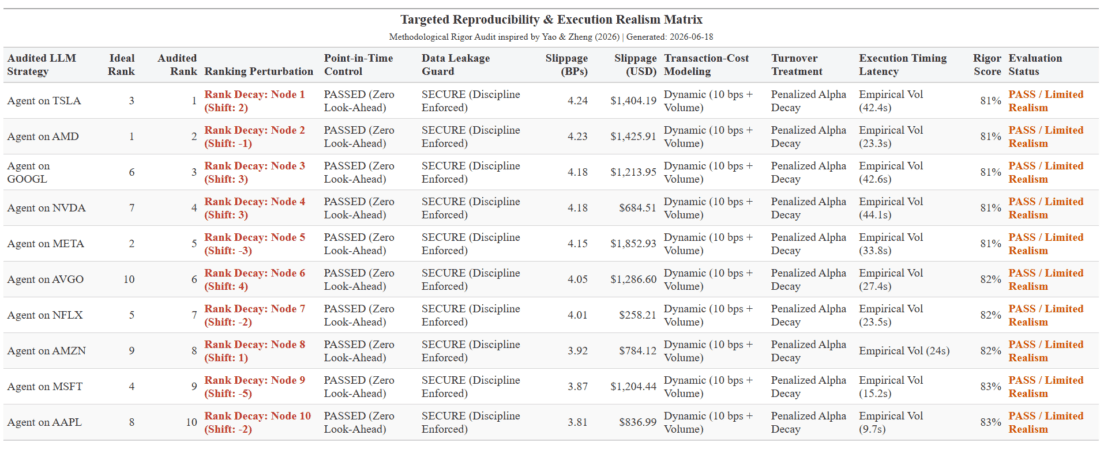

Source: DataGeeek

Conclusion: Reclaiming Empirical Rigor

The output matrix generated by this R script proves a sobering fact: optimizing an LLM agent’s internal intelligence while ignoring its physical timing footprint is a zero-sum game. When cognitive latency meets volatile market microstructure, theoretical priority hierarchies collapse.

By pushing dynamic slippage parameters directly into your research data layer rather than treats them as a post-trade footnote, you can accurately strip away laboratorial illusion. Quantitative researchers must stop asking how smart their financial agents are, and start measuring how fast those agents’ decisions decay on the trade desk.

From Theory to Production: Deploy the Audit Engine

While this analysis details the mathematical framework and the visual execution matrix of structural market breaks, implementing Yao & Zheng (2026) within a live trading infrastructure requires a robust, isolated, and highly integrated microservice architecture.

Visit DataGeeek blog for additional insights on this topic.