Options Indicators

Executive summary — Options activity embeds information and pressure that can forecast equities at horizons from one day to several months. In this article we explore four recurring mechanisms: (i) asymmetric information (informed traders choose options when shorting stock is costly), (ii) embedded leverage (OTM contracts amplify informed views), (iii) hedging demand (delta/gamma hedgers push underlying prices temporarily), and (iv) crowd‑level imbalance (ratios of option to stock trading, skew, and moneyness mix). These mechanisms translate into robust, implementable stock‑level predictors.

We then uncover how Visual Sectors have constructed Options Indicators, the step by step process and backtest results

Options trading vs Options data

Options are risky to trade, but the footprints they leave—volume, moneyness, order type, and hedging pressure—are a gold mine for signals about where the underlying stock is headed next. This idea isn’t new; it’s been explored for decades, from classic asymmetric‑information models to modern microstructure measures that use real‑time Greeks. What’s changed is data quality and scale: options activity is now large enough that its own flows and hedges can move stocks—creating short‑lived, tradable predictability.

After exchange‑traded equity options launched in 1973, researchers asked a simple question: do informed traders migrate to options to express views more precisely or with leverage? Theory says yes, especially when options allow better alignment with the sign/magnitude of private information. That thesis matured into testable signals:

• Relative option activity vs. stock activity (O/S): When shorting stock is costly, negative information is more likely to show up in options trading first, making high O/S bearish in the cross‑section. Empirically, going long low‑O/S and short high‑O/S names earns about 1.47% next‑month alpha in U.S. equities, and the effect is stronger where short‑sale frictions are higher. (“provide an average risk‑adjusted hedge return of 1.47% in the month following the formation date.”) [1]
• Where in the options chain do informed traders trade? Evidence shows they favor higher‑leverage contracts (OTM calls for bullish news; OTM puts for bearish), and that weighted average moneyness has forecasting power for next‑day and next‑month returns—especially in high‑IV names. (“Stock returns increase with this measure.”) [2]
• Who’s trading? Using order‑type/trader‑type data, customer “opening buy” flow dominates option volume and is particularly predictive, consistent with earlier work showing that customer (full‑service) order flow leads stock moves. (“specific market participant’s options trading volume is a predecessor to asset price movements.”) [3]
• Hedging pressure as a driver: With options volume and O/S ratios much larger than in the 1990s, market‑maker delta‑hedging itself has become a short‑horizon return driver. A new measure—Expected Hedging Demand (EHD) built from Greeks—predicts higher 1–5 day returns, followed by reversal, consistent with price pressure, not long‑horizon information. (“the positive impact … lasts up to five trading days, and then a reversal follows.”) [4]

The upshot: options data are not a novelty. They have been scrutinized theoretically and empirically, with practical, repeatable signals emerging across four mechanisms that matter most.

Factor 1 – Asymmetric information

Concept. When some traders know more, they prefer venues that let them size bets to information. Options offer sign‑targeted exposure (calls/puts) and embedded leverage. If shorting stock is costly, negative information migrates to options markets.

How it works. Contrast total options volume with stock volume for the same firm (the O/S ratio). In a multimarket microstructure model with short‑sale costs and capital constraints, informed traders disproportionately use options to act on bad news. That makes O/S a negative cross‑sectional signal for next‑period stock returns. Empirically, sorting monthly on O/S and going long the bottom decile vs. short the top decile delivers ~1.47% next‑month 5‑factor alpha, concentrated in the first few trading days; the effect fades by month two.

“Portfolio alphas associated with O/S are increasing in the cost of shorting.” (limits‑to‑shorting sharpen the signal). [5]

Why it’s legit. This is about where informed traders route orders given frictions. The same paper also shows the O/S signal weakens when options’ effective leverage (and spreads) are very high—because wider spreads deter switching from equities to options for negative signals.

Limitations. It’s a short‑horizon signal (days to ~1 month). And because it relies on public, unsigned totals, it’s strongest where shorting is hard; in easy‑to‑short names, the edge compresses.

How to use it. Compute each stock’s options volume (5–35 trading‑day maturities) divided by equity volume; rebalance monthly; emphasize stocks with high short‑sale fees/low lendable supply.

Factor 2 — Hedging demand

Concept. Today’s options market is big enough that delta‑hedging flows can push the underlying. When option makers collectively need to buy (sell) stock to hedge, that creates mechanical, short‑lived price pressure.

How it works. Expected Hedging Demand (EHD) uses real‑time Greeks to estimate how much hedging the options book will need (via elasticity of delta, ED = Γ·S/Δ, aggregated across open interest). High EHD today predicts higher stock returns over ~1–5 days, which then reverse—a signature of transitory demand.

“EHD significantly predicts future stock returns in the cross section … [and] the positive impact … lasts up to five trading days, and then a reversal follows.”[4]

This effect remains after controls and is economically meaningful (roughly double‑digit annualized when scaled by realistic turnover in deciles), and it is distinct from classic characteristics (size, spreads, volume) per cross‑sectional regressions and double‑sorts.

Limitations. It’s very short‑term and can invert across stocks with extremely high ED (elastic demand curves dampen net price impact). Implementation is data‑ and compute‑heavy (intra‑day Greeks, open interest).

How to use it. Build a daily EHD from OptionMetrics/Greeks by contract, open‑interest‑weighted to the firm day; buy high‑EHD names for hours–days; expect mean reversion beyond a week.

Factor 3 — Embedded leverage (signal in where activity concentrates on the chain)

Concept. If informed traders prefer higher‑leverage options, the distribution of trading across moneyness is itself informative.

How it works. Construct AveMoney: a dollar‑volume‑weighted average of K/S across a stock’s traded options. Higher AveMoney (more activity in higher‑strike calls, i.e., further OTM calls) predicts higher next‑day (and, for high‑IV names, next‑month) returns. The effect is strongest when implied volatility is high and when open interest is growing, consistent with informed risk‑taking rather than pure hedging.

“Stock returns increase with this measure.” (AveMoney). A long‑high vs. short‑low AveMoney (calls) portfolio delivers “a five‑factor alpha of 12% per year”—and ~33% per year in high‑IV stocks. [2]

Limitations. Put‑side patterns are noisier (puts are often hedges); the cleanest edge is on call‑side AveMoney and in high‑IV cohorts. Turnover and transaction costs matter for daily rebalancing.

How to use it. Each day:

(1) compute AveMoney=Σ(K/S)×(mid×volume)/Σ(mid×volume) \text{AveMoney}=\sum (K/S)\times \text{(mid×volume)} / \sum (\text{mid×volume})AveMoney=Σ(K/S)×(mid×volume)/Σ(mid×volume);

(2) sort on call‑only AveMoney;

(3) long high‑AveMoney, short low‑AveMoney;

(4) focus on high‑IV buckets and on days with rising open interest.

Factor 4 — Crowd wisdom (options‑based sentiment from who is buying what)

Concept. “Wisdom of crowds” in options is measurable via put‑call ratios—if you filter by order type and trader type to capture investor sentiment rather than market‑maker inventory.

How it works. Using ISE’s trader‑segmented data, customer “opening buy” flow dominates and is predictive; strategies that rank stocks by customer call‑to‑put ratios and go long the most bullish/short the most bearish deliver risk‑adjusted excess returns. The authors put it plainly: “specific market participant’s options trading volume is a predecessor to asset price movements.” [3]

The paper also documents who drives activity—customer traders account for ~67% of opening‑buy call volume and ~63% for puts—and notes prior evidence that such “full‑service” (customer) flow was the most reliable predictor of future gains. The diagram on page 4 (“Breakdown of ISE Option Data”) shows the pipeline from order type → trader type → put/call → ratio, making the sentiment construction transparent.

Limitations. Aggregate PCRs can be contrarian at extremes and blend stock‑specific with market‑wide fear. Trader‑segmented PCRs are stronger but require specialized feeds.

How to use it. Prefer customer “opening buy” PCRs at the single‑name level; weight by minimum volume (e.g., ≥50 contracts) to avoid micro‑prints; rebalance daily.

Pulling it together: when options data works best

1. Near catalysts or earnings: O/S and moneyness activity tend to anticipate the sign and magnitude of near‑term news.
2. Where shorting is hard: O/S is strongest when short‑sale costs and loan fees are high.
3. High implied‑volatility cohorts: Call‑side moneyness concentration has its biggest edge here.
4. High hedging intensity: Large, same‑day EHD spikes create 1–5 day drifts (then reversal).

Bottom line: Trading options may be risky, but options data—O/S, hedging demand, moneyness concentration, and trader‑segmented sentiment—consistently improves prediction of short‑horizon stock moves. The edges are real, researched, and replicable with clean data and careful cost control.

Visual Sectors case study

At Visual Sectors our mission is to help retail investors busy with their day to day chores find edge using new approaches and strictly data-based research.

So having learned all the above about options information, we decided to create indicators that would have very clear use cases, backtested performance metrics and wouldn’t take much time to implement in strategies.

Let’s explore the process of creating one of the indicators – Accumulation change indicator (ACI)

The logic behind this indicator is to grasp the general sentiment for equity. We wanted to use delta-adjusted open interest to define whether the sentiment is bullish or bearish.

Feature engineering: factors in play

First of all, we looked at our sentiment map to actually try and spot recurring patterns

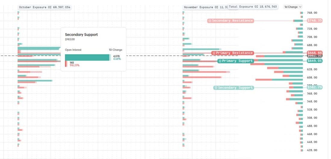
Source: Visual Sectors

Delta-adjusted OI is displayed within 2 buckets – bullish and bearish
We quantify daily, 5 day, 30 day change by expiration, strike and total

So to engineer features of the new indicator we had the following options to explore:

1. Days till expiration (DTE): if grouped by time, which group has the best predictive power? We ignored anything less than 5 DTE because theta made options prices change too rapidly. This wouldn’t work for swing traders placing directional trades
   
   The buckets for testing we want with:
   • 5-15 DTE
   • 16-30 DTE
   • 31 – 45 DTE
   • 46 – 60 DTE
2. Moneyness: how “far” in the money or out of the money open positions have predictive power? If a stock has bets with 500% upside – do we actually think it’s a valid price target? Probably not. So we can choose to ignore it.
   
   The straightforward way to calculate moneyness is to apply 100% to current stock price and just measure how far the strike is from current price.
   
   However, not all stocks have a similar range of trades. Some would only move by 10% a month, other – more than 50%. Also, we noticed the dispersion of open interest wasn’t similar too. Some very popular stocks could have a massive bulk of open interest 200-300% out of the money (for calls), smaller stocks with less open interest could have all of it accumulated within several per cent of the current price.
   
   So we decided to test traditional moneyness calculation, but also, OI weighted.
   
   The idea is to focus on the large chunks of open interest and define strikes that fall within a bucket of 60%, 70%, 80% or 90% of open interest. So we can actually pay attention to flexible ranges, like 80% through 150% of the current price for calls for 1 stock compared to 90-110% for another stock.
3. Holding and analysis period: how many days of Open interest change should we track? When should we sell?
   
   It’s actually pretty straightforward. Delta-adjusted open interest change over 1 trading session, 2, 3, 4, 5 (aka 1 calendar week), 2 and 3 weeks. Same for holding periods. If you buy the equity using this indicator – how long should you hold it before selling?
   
   It gives us 49 possible combinations to backtest
4. Weekday: is there a difference between buying on Tuesdays or on Fridays? Funny enough, there is. So we decided to add 6 more variants: “any day” + 5 weekdays
   

All those factors and the variants of the indicator to backtest summed up to 9,408 backtests that needed to be run for each stock. Our data covers a universe of 3,455 stocks.

Backtesting challenges

We needed to make several other decisions like: which period does the backtest have to cover? What performance metrics are the priority? Should we add stop-loss/take-profit rules?

1. Defining the period was pretty straightforward. The idea that the market has changed post-COVID (but really – post-2018 panic rate cuts) pretty much defined the depth of the tests. But we also didn’t want the “helicopter money” of post-COVID bounce back distorting results. So we chose January 1st, 2022 at the starting point and April 30th 2025 as the end date. This period has 2 very distinct bear markets and an extended bull market with 2 different regimes (low and high volatility market expansion)

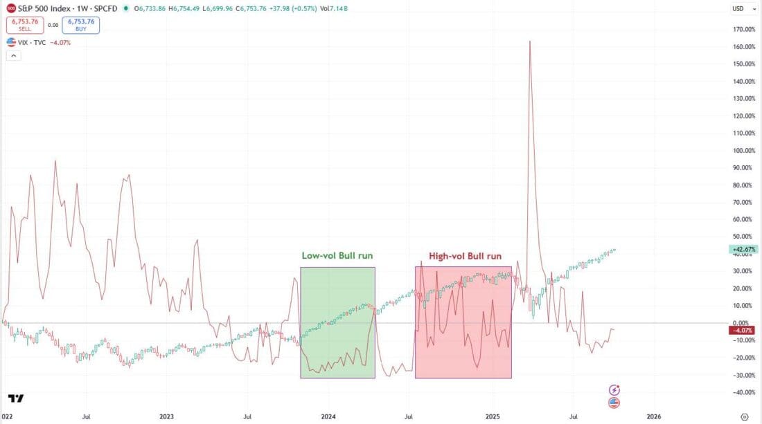
Source: Tradingview

2. Take-profit and stop-loss

One of the big questions for a “calendar” defined system is obviously: what if the price makes a rapid move? Either in your favor or not, do you keep holding?

So we took all the positive records (price going the predicted direction) and all the negative records (price going the wrong way) and ran a quick backtest to see how often it reverses, and from what levels. Empirically, we identified 60th percentile for take profit and 40th percentile for stop loss.

Basically, we ignore the top 40% of the best moves for the sake of keeping what 60% of price moves can lock in profit. Same way: if we see a price move that’s within 40% smallest losses, we cut and don’t sit out larger drawdowns.

Perhaps, we can further explore these rules but for now – it’s a switch on/off mode to double the amount of backtests mentioned above: with take profit and stop loss or just according to the calendar.

3. Performance metrics

We focused on indicator variants that returned at least 40 observations across the 40 month backtest period. The argument for the priority metric internally was heated so we decided to let everyone decide for themselves and created simple filters and sorted columns of:

1. $1,000 invested (only invest $1,000 per trade)
2. Annualised cumulative return (reinvest profit)
3. Win rate by trade (% of profitable trades)
4. Win rate by month (% of profitable months)
5. Alpha compared to broad market index
6. Reward:Risk: median losing trade loss vs average winning trade win
7. Sharpe ratio
8. Sortino ratio
9. Latency to profit (how many trading sessions would it take to get into positive returns)
10. Hit and Loss streaks (how many losing/profitable trades in a row have been recorded at its maximum)
11. Win 3 out of 4 probability – something to keep your chin up, out of any random 4 trades in a row, what’s the chance to see 3 profitable?
12. Maximum drawdown

All of those are calculated for buy and hold for set days and for take profit/stop loss

4. Overfitting

To avoid overfitting we decided to return results not just for the whole period of 40 months but also separately for:

• Bull markets
• Bear markets
• Full calendar years of 2022, 2023,2024 and 4 months of 2025

Winning combinations for each stock would display the full period results, but filter out variants where even one of the mentioned above periods would underperform significantly. The borderline requirement was to return 10% annually, have a 55% month win rate, max drawdown less than 10% per trade.

Results overview

The amount of results was overwhelming, so we used Google’s LookerStudio to display them

The variables would act as filters:

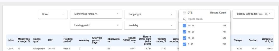
Performance metrics would be displayed as columns:

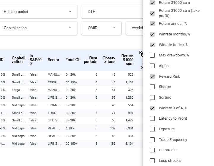
Source: Visual Sectors

And each stock would open a breakdown by periods:

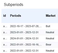
Source: Visual Sectors

So here are our winners:

• CLF for winning months %

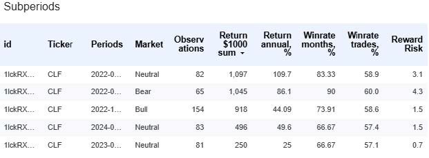
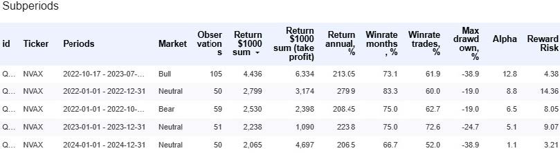
Source: Visual Sectors

• NVAX for return on $1,000 invested

Source: Visual Sectors