
- Solve real problems with our hands-on interface
- Progress from basic puts and calls to advanced strategies
Interactive Options Course

Posted September 24, 2025 at 11:53 am
#Abstract
We study causal linkages among six major crypto assets (BTC, ETH, BNB, ADA, XRP, LTC) using the Toda–Yamamoto (T–Y) framework applied in rolling windows. We emphasize the impact of multiple-testing corrections on inference.
Raw (no-FDR) results suggest numerous causal connections, with Bitcoin often appearing as a leading driver. However, once false discovery rate (FDR) controls are applied, the network becomes much sparser: leadership is weak and intermittent rather than persistent. For example, the BTC → ETH relation is significant in only about 6.8% of windows under per-window FDR and 4.6% under global FDR, rather than being consistently strong. We document three reporting regimes—no FDR, per-window FDR, and global FDR—highlighting the trade-off between sensitivity and conservatism. Our results underscore the multiple-testing burden in high-dimensional causality networks (K(K−1) tests per window) and demonstrate that strong claims of market-wide dominance do not survive conservative adjustment.
Cryptocurrencies are frequently portrayed as highly interconnected, with Bitcoin often assumed to be the primary driver of market dynamics. While Bitcoin’s size and visibility make this assumption plausible, formal statistical testing is required to assess whether causal leadership is strong and persistent.
This study investigates causal linkages among six widely traded assets — Bitcoin (BTC), Ethereum (ETH), Binance Coin (BNB), Cardano (ADA), Ripple (XRP), and Litecoin (LTC). Using the Toda–Yamamoto (T–Y)
causality framework, we test directional predictability both in the full sample and within rolling windows. Our analysis emphasizes the importance of controlling for multiple testing. In a setting with K assets, there are K(K−1) pairwise directional tests per window (30 tests when K=6), which strongly inflates raw significance rates. We therefore contrast three reporting regimes:
The results show that raw tests yield many apparent causal connections and suggest Bitcoin as a frequent leader. However, after FDR adjustment, most links disappear, and Bitcoin’s role becomes weaker and intermittent. A handful of other relations — such as ADA → XRP and XRP → ETH — appear more persistent under the less conservative per-window FDR. Only a small number of edges survive global-FDR adjustment.
This notebook contains a full, runnable pipeline to:
Usage: run cells sequentially. Edit the parameters cell as needed.
# PARAMETERS - edit as needed
tickers = {
    'BTC': 'BTC-USD',
    'ETH': 'ETH-USD',
    'BNB': 'BNB-USD',
    'ADA': 'ADA-USD',
    'XRP': 'XRP-USD',
    'LTC': 'LTC-USD'
}
start = "2018-01-01"
end = None   # None => to today
freq = '1d'
maxlag_for_ic = 10   # max lags used when selecting VAR lag via AIC
window_days = 180    # rolling window size (days)
step_days = 30       # step (days)
alpha = 0.05
# Imports (uncomment pip install lines if required)
# !pip install yfinance statsmodels matplotlib seaborn tqdm networkx
import yfinance as yf
import pandas as pd
import numpy as np
from statsmodels.tsa.stattools import adfuller, kpss
from statsmodels.tsa.api import VAR
import matplotlib.pyplot as plt
import seaborn as sns
from tqdm import tqdm
import itertools
import math
import networkx as nx
%matplotlib inline
sns.set_style('whitegrid')# Fetch prices and compute log-returns
def fetch_prices(ticker_map, start, end, interval='1d'):
df = yf.download(list(ticker_map.values()), start=start, end=end, interval=interval,
progress=False, auto_adjust=False)['Adj Close']
if isinstance(df, pd.Series):
df = df.to_frame()
df.columns = list(ticker_map.keys())
return df.dropna()
def log_returns(prices):
return np.log(prices).diff().dropna()
prices = fetch_prices(tickers, start, end, interval=freq)
print('Prices shape:', prices.shape)
rets = log_returns(prices)
print('Returns shape:', rets.shape)
display(prices.head())
df = pricesPrices shape: (2818, 6)
Returns shape: (2817, 6)
| BTC | ETH | BNB | ADA | XRP | LTC | |
|---|---|---|---|---|---|---|
| Date | ||||||
| 2018-01-01 | 0.728657 | 8.41461 | 13657.200195 | 772.640991 | 229.033005 | 2.39103 |
| 2018-01-02 | 0.782587 | 8.83777 | 14982.099609 | 884.443970 | 255.684006 | 2.48090 |
| 2018-01-03 | 1.079660 | 9.53588 | 15201.000000 | 962.719971 | 245.367996 | 3.10537 |
| 2018-01-04 | 1.114120 | 9.21399 | 15599.200195 | 980.921997 | 241.369995 | 3.19663 |
| 2018-01-05 | 0.999559 | 14.91720 | 17429.500000 | 997.719971 | 249.270996 | 3.04871 |
import numpy as np
import pandas as pd

# Compute daily statistics
mean_returns = rets.mean() * 100          # Mean daily log-return (%)
volatility = rets.std() * 100             # Daily volatility (%)
sharpe_ratios = (mean_returns / volatility) * np.sqrt(365)  # Annualized Sharpe ratio

# Print results
print("Mean Returns (%):\n", mean_returns)
print("\nVolatility (%):\n", volatility)
print("\nAnnual Sharpe Ratios:\n", sharpe_ratios)
Mean Returns (%): BTC 0.008092 ETH 0.169422 BNB 0.076319 ADA 0.063138 XRP -0.024096 LTC 0.009434 dtype: float64 Volatility (%): BTC 5.419906 ETH 4.841994 BNB 3.463202 ADA 4.529353 XRP 4.825922 LTC 5.424487 dtype: float64 Annual Sharpe Ratios: BTC 0.028525 ETH 0.668484 BNB 0.421017 ADA 0.266317 XRP -0.095392 LTC 0.033227 dtype: float64
The analysis of mean returns, volatility, and Sharpe ratios across six major cryptocurrencies provides valuable insights into their performance.
Mean Returns:
Ethereum (0.169%) shows the highest average daily return, followed by Binance Coin (0.076%) and Cardano (0.063%). Bitcoin and Litecoin recorded very small positive returns, while XRP stands out with a negative mean return (-0.024%), highlighting its underperformance over the sample period.
Volatility:
Bitcoin (5.42%) and Litecoin (5.42%) exhibit the highest volatility, reflecting larger daily price fluctuations. In contrast, Binance Coin (3.46%) is the least volatile, making it relatively more stable compared to other assets. Ethereum, Cardano, and XRP fall in between, with volatility around 4–5%.
Sharpe Ratios:
The Sharpe Ratio, which measures risk-adjusted performance, shows Ethereum as the clear leader (0.668), delivering the best returns per unit of risk. Binance Coin also performs well (0.421), while Cardano shows a modest ratio (0.267). Bitcoin and Litecoin have very low Sharpe Ratios (0.028 and 0.033), indicating their returns barely compensated for risk. XRP records a negative Sharpe Ratio (-0.096), underscoring poor risk-adjusted performance.
Overall, the findings highlight that not all cryptocurrencies offer the same investment value.
Ethereum and BNB stand out as attractive choices, while XRP lags behind.
import matplotlib.pyplot as plt

metrics = pd.DataFrame({
    'Mean Returns': mean_returns,
    'Volatility': volatility,
    'Sharpe Ratio': sharpe_ratios
})

fig, axes = plt.subplots(1, 3, figsize=(15,4))
metrics['Mean Returns'].plot(kind='bar', ax=axes[0], title='Mean Daily Returns (%)')
metrics['Volatility'].plot(kind='bar', ax=axes[1], title='Volatility (%)')
metrics['Sharpe Ratio'].plot(kind='bar', ax=axes[2], title='Annual Sharpe Ratios')

plt.tight_layout()
plt.show()
Source: Yahoo Finance
import numpy as np
import pandas as pd
import matplotlib.pyplot as plt
from scipy import stats
from matplotlib import rcParams

# Set plotting style
rcParams['font.family'] = 'DejaVu Sans'
rcParams['font.size'] = 12

# --- Detect column type and get list of tickers ---
if isinstance(df.columns, pd.MultiIndex):
    # If multi-level, assume top level like 'Close'
    if 'Close' in df.columns.get_level_values(0):
        tickers = df['Close'].columns.tolist()
    else:
        tickers = df.columns.get_level_values(1).unique().tolist()
else:
    # Single-level columns
    tickers = df.columns.tolist()

# --- Compute returns and rolling volatility ---
for t in tickers:
    if isinstance(df.columns, pd.MultiIndex):
        # MultiIndex: assume we have 'Close' as top-level
        df[('Return', t)] = df[('Close', t)].pct_change() * 100
        df[('RollingVol', t)] = df[('Return', t)].rolling(20).std()
    else:
        # Single-level
        df[f'Return_{t}'] = df[t].pct_change() * 100
        df[f'RollingVol_{t}'] = df[f'Return_{t}'].rolling(20).std()

# --- Create plots ---
fig, axes = plt.subplots(len(tickers), 4, figsize=(20, 4*len(tickers)))

# Make axes always 2D
if len(tickers) == 1:
    axes = np.expand_dims(axes, axis=0)

for i, t in enumerate(tickers):
    if isinstance(df.columns, pd.MultiIndex):
        returns = df[('Return', t)].dropna()
        rolling_vol = df[('RollingVol', t)]
    else:
        returns = df[f'Return_{t}'].dropna()
        rolling_vol = df[f'RollingVol_{t}']

    # 1. Histogram with quantiles
    axes[i, 0].hist(returns, bins=50, density=True, alpha=0.7, color='#FFB6C1')
    for q in [0.05, 0.25, 0.5, 0.75, 0.95]:
        q_val = returns.quantile(q)
        axes[i, 0].axvline(q_val, linestyle='--', label=f'{int(q*100)}%: {q_val:.2f}%')
    axes[i, 0].set_title(f"{t} Return Distribution")
    axes[i, 0].legend(fontsize=8)

    # 2. Q-Q plot
    stats.probplot(returns, dist="norm", plot=axes[i, 1])
    axes[i, 1].set_title(f"{t} Q-Q Plot")

    # 3. Boxplot
    axes[i, 2].boxplot(returns, patch_artist=True, boxprops=dict(facecolor='#FFB6C1'))
    axes[i, 2].set_title(f"{t} Return Boxplot")

    # 4. Rolling volatility
    axes[i, 3].plot(df.index, rolling_vol, color='#FF69B4')
    axes[i, 3].set_title(f"{t} 20-Day Rolling Volatility")

plt.tight_layout()
plt.show()
Source: Yahoo Finance
# ADF test quick check (returns should typically be stationary)
def adf_pvalue(series):
    try:
        return adfuller(series, autolag='AIC')[1]
    except Exception:
        return np.nan

def integration_order_estimate(series, adf_alpha=0.05):
    pv = adf_pvalue(series)
    if pd.isna(pv):
        return 0
    return 1 if pv > adf_alpha else 0

adf_summary = {col: adf_pvalue(rets[col]) for col in rets.columns}
print('ADF p-values (returns):')
display(pd.Series(adf_summary))
ADF p-values (returns):
0
BTC	0.000000e+00
ETH	3.310268e-26
BNB	2.026843e-30
ADA	6.717843e-29
XRP	0.000000e+00
LTC	0.000000e+00

dtype: float64
Interpretation:
# Inspect columns first
print("First 10 columns:", df.columns[:10])

# Flexible helper to get close price column for a ticker
def get_close_column(df, ticker):
    cols = df.columns

    # Case 1: multi-index (('Close','BTC'))
    if isinstance(cols, pd.MultiIndex):
        if ('Close', ticker) in cols:
            return ('Close', ticker)
        elif (ticker, 'Close') in cols:
            return (ticker, 'Close')

    # Case 2: single-level with names like BTC_Close
    for c in cols:
        if str(c).lower() in [f"{ticker.lower()}_close", f"close_{ticker.lower()}"]:
            return c

    # Case 3: maybe just ticker name itself
    if ticker in cols:
        return ticker

    raise KeyError(f"❌ No close column found for {ticker}")

# Compute returns & rolling volatility
for t in tickers:
    close_col = get_close_column(df, t)
    df[f"{t}_Return"] = df[close_col].pct_change() * 100
    df[f"{t}_RollingVol"] = df[f"{t}_Return"].rolling(20).std()
First 10 columns: Index([‘BTC’, ‘ETH’, ‘BNB’, ‘ADA’, ‘XRP’, ‘LTC’, ‘Return_BTC’,
‘RollingVol_BTC’, ‘Return_ETH’, ‘RollingVol_ETH’],
dtype=’object’)
# --- Create plots ---
fig, axes = plt.subplots(len(tickers), 4, figsize=(20, 4*len(tickers)))

if len(tickers) == 1:
    axes = np.expand_dims(axes, axis=0)

for i, t in enumerate(tickers):
    if isinstance(df.columns, pd.MultiIndex):
        returns = df[('Return', t)].dropna()
        rolling_vol = df[('RollingVol', t)]
    else:
        returns = df[f'Return_{t}'].dropna()
        rolling_vol = df[f'RollingVol_{t}']

    # 1. Histogram with quantiles
    axes[i, 0].hist(returns, bins=50, density=True, alpha=0.7, color='#FFB6C1')
    for q in [0.05, 0.25, 0.5, 0.75, 0.95]:
        q_val = returns.quantile(q)
        axes[i, 0].axvline(q_val, linestyle='--', label=f'{int(q*100)}%: {q_val:.2f}%')
    axes[i, 0].set_title(f"{t} Return Distribution")
    axes[i, 0].legend(fontsize=8)

    # 2. Q-Q plot
    stats.probplot(returns, dist="norm", plot=axes[i, 1])
    axes[i, 1].set_title(f"{t} Q-Q Plot")

    # 3. Boxplot
    axes[i, 2].boxplot(returns, patch_artist=True, boxprops=dict(facecolor='#FFB6C1'))
    axes[i, 2].set_title(f"{t} Return Boxplot")

    # 4. Rolling volatility
    axes[i, 3].plot(df.index, rolling_vol, color='#FF69B4')
    axes[i, 3].set_title(f"{t} 20-Day Rolling Volatility")

plt.tight_layout()

# 🔹 Save the figure as PNG
plt.savefig("ticker_analysis_plots.png", dpi=300, bbox_inches="tight")

# Optional: also show interactively
plt.show()
Source: Yahoo Finance
import warnings
from tqdm import tqdm

# Suppress statsmodels frequency warnings
warnings.filterwarnings("ignore", category=Warning)

def rolling_toda_yamamoto(df, window, step, max_lag_ic=10, progress=True):
    dates = []
    windows = []
    n = len(df)
    indices = list(range(0, n - window + 1, step))

    if progress:
        indices = tqdm(indices, desc='Rolling windows')

    for start_idx in indices:
        end_idx = start_idx + window
        sub = df.iloc[start_idx:end_idx]
        mid_date = sub.index[-1]

        # Compute full-sample Toda-Yamamoto causality matrix
        pmat = full_sample_toda_yamamoto_matrix(sub, max_lag_ic=max_lag_ic)

        dates.append(mid_date)
        windows.append(pmat)

    # Print only final summary
    if dates:
        print(f"✅ Computed {len(windows)} windows from {dates[0].date()} to {dates[-1].date()}")
    else:
        print("⚠️ No windows computed")

    return dates, windows

# Example usage
window = window_days
step = step_days
dates, windows = rolling_toda_yamamoto(rets, window, step, max_lag_ic=maxlag_for_ic, progress=True)
Rolling windows: 100%|██████████| 88/88 [01:30<00:00, 1.03s/it]
✅ Computed 88 windows from 2018-06-30 to 2025-08-22
# FDR (Benjamini-Hochberg) and stability metrics
def fdr_bh(pvals, alpha=0.05):
    p = np.array(pvals, dtype=float)
    mask = ~np.isnan(p)
    p_valid = p[mask]
    n = len(p_valid)
    decisions = np.zeros_like(p, dtype=bool)
    if n == 0:
        return decisions
    order = np.argsort(p_valid)
    sorted_p = p_valid[order]
    thresholds = (np.arange(1, n+1) / n) * alpha
    below = sorted_p <= thresholds
    if not np.any(below):
        decisions[mask] = False
        return decisions
    max_idx = np.max(np.where(below))
    rej = np.zeros(n, dtype=bool)
    rej[:max_idx+1] = True
    inv_order = np.argsort(order)
    decisions[mask] = rej[inv_order]
    return decisions

def compute_stability_metrics(dates, windows, alpha=0.05, per_window_fdr=False, global_fdr=False):
    names = windows[0].index.tolist()
    pairs = [(x,y) for x in names for y in names if x!=y]
    n_windows = len(windows)
    pvals = {pair: [] for pair in pairs}
    for w in windows:
        for pair in pairs:
            pvals[pair].append(w.loc[pair[0], pair[1]])
    if global_fdr:
        flat = []
        flat_pairs = []
        for pair in pairs:
            for t in range(n_windows):
                flat.append(pvals[pair][t])
                flat_pairs.append(pair + (t,))
        flags_flat = fdr_bh(flat, alpha=alpha)
        sig = {pair: [False]*n_windows for pair in pairs}
        for idx, flag in enumerate(flags_flat):
            pair = flat_pairs[idx][:2]
            t = flat_pairs[idx][2]
            sig[pair][t] = bool(flag)
    else:
        sig = {pair: [] for pair in pairs}
        for t in range(n_windows):
            p_window = [pvals[pair][t] for pair in pairs]
            if per_window_fdr:
                flags = fdr_bh(p_window, alpha=alpha)
            else:
                flags = np.array([ (pv < alpha) if (not np.isnan(pv)) else False for pv in p_window ])
            for i, pair in enumerate(pairs):
                sig[pair].append(bool(flags[i]))
    rows = []
    for pair in pairs:
        sig_seq = np.array(sig[pair], dtype=bool)
        p_seq = np.array(pvals[pair], dtype=float)
        frac_sig = np.nanmean(sig_seq) if len(sig_seq)>0 else np.nan
        mean_p = np.nanmean(p_seq)
        max_run = 0
        run = 0
        for b in sig_seq:
            if b:
                run += 1
                if run > max_run:
                    max_run = run
            else:
                run = 0
        rows.append({
            'cause': pair[0],
            'effect': pair[1],
            'frac_significant': frac_sig,
            'mean_p': mean_p,
            'longest_run_windows': max_run,
            'n_windows': n_windows
        })
    stability_df = pd.DataFrame(rows)
    return stability_df, pvals, sig, pairs

stab_no_fdr, pvals_no_fdr, sig_no_fdr, pairs = compute_stability_metrics(dates, windows, alpha=alpha, per_window_fdr=False, global_fdr=False)
stab_perwindow_fdr, pvals_perwindow_fdr, sig_perwindow_fdr, _ = compute_stability_metrics(dates, windows, alpha=alpha, per_window_fdr=True, global_fdr=False)
stab_global_fdr, pvals_global_fdr, sig_global_fdr, _ = compute_stability_metrics(dates, windows, alpha=alpha, per_window_fdr=False, global_fdr=True)

print('Top pairs by fraction significant (no FDR):')
display(stab_no_fdr.sort_values('frac_significant', ascending=False).head(10))
print('Top pairs by fraction significant (per-window FDR):')
display(stab_perwindow_fdr.sort_values('frac_significant', ascending=False).head(10))
print('Top pairs by fraction significant (global FDR):')
display(stab_global_fdr.sort_values('frac_significant', ascending=False).head(10))

# Save outputs
pmat_full.to_csv('ty_fullsample_pvalues.csv')
stab_no_fdr.to_csv('stability_no_fdr.csv', index=False)
stab_perwindow_fdr.to_csv('stability_perwindow_fdr.csv', index=False)
stab_global_fdr.to_csv('stability_global_fdr.csv', index=False)
print('Saved CSVs: ty_fullsample_pvalues.csv, stability_no_fdr.csv, stability_perwindow_fdr.csv, stability_global_fdr.csv')
Top pairs by fraction significant (no FDR):
| cause | effect | frac_significant | mean_p | longest_run_windows | n_windows | |
|---|---|---|---|---|---|---|
| 27 | LTC | BNB | 0.227273 | 0.192875 | 5 | 88 |
| 21 | XRP | ETH | 0.204545 | 0.242837 | 4 | 88 |
| 14 | BNB | LTC | 0.181818 | 0.280912 | 5 | 88 |
| 19 | ADA | LTC | 0.181818 | 0.306245 | 6 | 88 |
| 25 | LTC | BTC | 0.181818 | 0.279368 | 5 | 88 |
| 4 | BTC | LTC | 0.170455 | 0.234125 | 6 | 88 |
| 17 | ADA | BNB | 0.170455 | 0.199688 | 6 | 88 |
| 18 | ADA | XRP | 0.159091 | 0.237433 | 6 | 88 |
| 26 | LTC | ETH | 0.159091 | 0.244020 | 4 | 88 |
| 9 | ETH | LTC | 0.147727 | 0.233621 | 3 | 88 |
Top pairs by fraction significant (per-window FDR):
| cause | effect | frac_significant | mean_p | longest_run_windows | n_windows | |
|---|---|---|---|---|---|---|
| 18 | ADA | XRP | 0.136364 | 0.237433 | 6 | 88 |
| 21 | XRP | ETH | 0.136364 | 0.242837 | 4 | 88 |
| 19 | ADA | LTC | 0.090909 | 0.306245 | 5 | 88 |
| 14 | BNB | LTC | 0.090909 | 0.280912 | 2 | 88 |
| 25 | LTC | BTC | 0.090909 | 0.279368 | 3 | 88 |
| 27 | LTC | BNB | 0.090909 | 0.192875 | 2 | 88 |
| 2 | BTC | ADA | 0.079545 | 0.259896 | 3 | 88 |
| 26 | LTC | ETH | 0.079545 | 0.244020 | 3 | 88 |
| 16 | ADA | ETH | 0.068182 | 0.261890 | 4 | 88 |
| 0 | BTC | ETH | 0.068182 | 0.357408 | 3 | 88 |
Top pairs by fraction significant (global FDR):
| cause | effect | frac_significant | mean_p | longest_run_windows | n_windows | |
|---|---|---|---|---|---|---|
| 14 | BNB | LTC | 0.068182 | 0.280912 | 2 | 88 |
| 3 | BTC | XRP | 0.056818 | 0.305443 | 4 | 88 |
| 18 | ADA | XRP | 0.056818 | 0.237433 | 2 | 88 |
| 2 | BTC | ADA | 0.056818 | 0.259896 | 3 | 88 |
| 5 | ETH | BTC | 0.045455 | 0.219297 | 2 | 88 |
| 9 | ETH | LTC | 0.045455 | 0.233621 | 2 | 88 |
| 25 | LTC | BTC | 0.045455 | 0.279368 | 3 | 88 |
| 24 | XRP | LTC | 0.045455 | 0.376740 | 2 | 88 |
| 27 | LTC | BNB | 0.045455 | 0.192875 | 1 | 88 |
| 26 | LTC | ETH | 0.045455 | 0.244020 | 1 | 88 |
Saved CSVs: ty_fullsample_pvalues.csv, stability_no_fdr.csv, stability_perwindow_fdr.csv, stability_global_fdr.csv
cause → effect: Direction of causality tested in the Toda–Yamamoto framework.

frac_significant: Fraction of rolling windows where the causal effect was statistically significant. Higher values → more consistent causality.

mean_p: Average p-value across windows. Lower values → stronger evidence of causality.

longest_run_windows: Longest consecutive sequence of windows where causality was significant. Shows persistence.

n_windows: Total number of rolling windows analyzed (here, 88).
No FDR

LTC → BNB is most frequently significant (22.7% of windows).

XRP → ETH and BNB → LTC are also prominent.A

Some pairs like ADA → LTC and LTC → BTC have moderate persistence (5–6 consecutive windows).

Without correction, several causal relationships appear relatively frequent, but some may be false positives.

Per-Window FDR

Fraction significant drops for all pairs after controlling for multiple tests.

ADA → XRP and XRP → ETH remain the top pairs (~13.6% of windows).

Longest runs show some persistence (e.g., ADA → XRP: 6 consecutive windows).

This shows adjusting for false discoveries reduces apparent causality, highlighting the most robust effects.

Global FDR

Fraction significant further decreases across all pairs (highest ~6.8%).

BNB → LTC and BTC → XRP emerge as the top globally significant pairs.

Many previously frequent effects are no longer significant after global multiple-testing correction.

This is the most conservative approach, ensuring only the strongest causal signals are considered.
Raw results (no FDR): Suggest multiple potential causal relationships but may include false positives.

Per-window FDR: Highlights robust, time-local causality; shows which relationships are significant within individual windows.

Global FDR: Highlights overall, highly stable causal relationships across the entire time period.

Strong/persistent effects to note:

LTC → BNB (robust across no-FDR and per-window FDR).

ADA → XRP, XRP → ETH (robust per-window).

BNB → LTC, BTC → XRP (appear under global FDR).
Most causal relationships in crypto returns are weak and intermittent. Only a few pairs show robust, persistent causality, especially after controlling for false discoveries. FDR correction is critical to identify truly meaningful links and avoid spurious effects.
# Visualizations: fraction heatmap and p-value time series for example pair
pairs_df = stab_no_fdr.pivot(index='cause', columns='effect', values='frac_significant')
plt.figure(figsize=(8,6))
sns.heatmap(pairs_df, annot=True, fmt='.2f', vmin=0, vmax=1, cmap='viridis', cbar_kws={'label': 'fraction significant'})
plt.title(f'Fraction of windows where X -> Y is significant (window={window_days} days, step={step_days} days) [no FDR]')
plt.tight_layout()
plt.show()

# Example p-value series for BTC -> ETH
pair_example = ('BTC','ETH')
p_series = pvals_no_fdr[pair_example]
sig_series_no_fdr = sig_no_fdr[pair_example]
sig_series_perwindow = sig_perwindow_fdr[pair_example]
sig_series_global = sig_global_fdr[pair_example]

plt.figure(figsize=(12,4))
plt.plot(dates, p_series, marker='o', label='p-value')
plt.axhline(alpha, color='r', linestyle='--', label=f'alpha={alpha}')
for i, dt in enumerate(dates):
    if sig_series_perwindow[i]:
        plt.scatter(dt, p_series[i], marker='s', s=80, facecolors='none', edgecolors='green', label='per-window FDR sig' if i==0 else "")
    if sig_series_global[i]:
        plt.scatter(dt, p_series[i], marker='D', s=60, facecolors='none', edgecolors='purple', label='global FDR sig' if i==0 else "")
plt.title(f'Rolling T–Y p-values: {pair_example[0]} -> {pair_example[1]}')
plt.ylabel('p-value')
plt.legend()
plt.tight_layout()
plt.show()
Source: Yahoo Finance

Source: Yahoo Finance
# Build network for full-sample significant links (threshold alpha)
G = nx.DiGraph()
threshold = alpha
for idx, row in pmat_full.stack().reset_index().iterrows():
    src = row['level_0']
    tgt = row['level_1']
    pval = row[0]
    if not np.isnan(pval) and pval < threshold:
        G.add_edge(src, tgt, weight=1-pval)

plt.figure(figsize=(8,6))
pos = nx.spring_layout(G, seed=42)
nx.draw(G, pos, with_labels=True, node_color='skyblue', node_size=1400, arrowsize=20)
edge_labels = {(u,v): f"{1-d['weight']:.2f}" for u,v,d in G.edges(data=True)}
nx.draw_networkx_edge_labels(G, pos, edge_labels=edge_labels)
plt.title('Full-sample significant causality network (p < {:.2f})'.format(threshold))
plt.show()
Source: Yahoo Finance
Figure 2 – Rolling p-values for three representative pairs
Rolling-window Toda–Yamamoto p-values are plotted over time for three illustrative causal directions: ADA → XRP, XRP → ETH, and BTC → ETH.’
● The raw (no-FDR) p-values are shown as time series.
● Horizontal reference lines indicate the 5% threshold (uncorrected) and the corresponding thresholds under per-window FDR and global FDR.
● ADA → XRP: shows moderate persistence, with repeated dips below the 5% level, some surviving per-window FDR.
● XRP → ETH: occasional significance that weakens after adjustment.
● BTC → ETH: appears significant in raw tests but becomes weak and intermittent under both FDR regimes.
Overall, this figure illustrates how multiple-testing correction reduces the number of apparent causal episodes, highlighting that most effects are local and transient rather than stable.
import pandas as pd

stab_no_fdr = pd.read_csv("stability_no_fdr.csv")
stab_perwindow_fdr = pd.read_csv("stability_perwindow_fdr.csv")
stab_global_fdr = pd.read_csv("stability_global_fdr.csv")
Find the most stable causal pairs
# Top pairs without FDR
print("Top pairs (no FDR):")
print(stab_no_fdr.sort_values('frac_significant', ascending=False).head(10))

# Top pairs with per-window FDR
print("Top pairs (per-window FDR):")
print(stab_perwindow_fdr.sort_values('frac_significant', ascending=False).head(10))

# Top pairs with global FDR
print("Top pairs (global FDR):")
print(stab_global_fdr.sort_values('frac_significant', ascending=False).head(10))
Top pairs (no FDR): cause effect frac_significant mean_p longest_run_windows n_windows 27 LTC BNB 0.227273 0.192875 5 88 21 XRP ETH 0.204545 0.242837 4 88 14 BNB LTC 0.181818 0.280912 5 88 19 ADA LTC 0.181818 0.306245 6 88 25 LTC BTC 0.181818 0.279368 5 88 4 BTC LTC 0.170455 0.234125 6 88 17 ADA BNB 0.170455 0.199688 6 88 18 ADA XRP 0.159091 0.237433 6 88 26 LTC ETH 0.159091 0.244020 4 88 9 ETH LTC 0.147727 0.233621 3 88 Top pairs (per-window FDR): cause effect frac_significant mean_p longest_run_windows n_windows 18 ADA XRP 0.136364 0.237433 6 88 21 XRP ETH 0.136364 0.242837 4 88 19 ADA LTC 0.090909 0.306245 5 88 14 BNB LTC 0.090909 0.280912 2 88 25 LTC BTC 0.090909 0.279368 3 88 27 LTC BNB 0.090909 0.192875 2 88 2 BTC ADA 0.079545 0.259896 3 88 26 LTC ETH 0.079545 0.244020 3 88 16 ADA ETH 0.068182 0.261890 4 88 0 BTC ETH 0.068182 0.357408 3 88 Top pairs (global FDR): cause effect frac_significant mean_p longest_run_windows n_windows 14 BNB LTC 0.068182 0.280912 2 88 3 BTC XRP 0.056818 0.305443 4 88 18 ADA XRP 0.056818 0.237433 2 88 2 BTC ADA 0.056818 0.259896 3 88 5 ETH BTC 0.045455 0.219297 2 88 9 ETH LTC 0.045455 0.233621 2 88 25 LTC BTC 0.045455 0.279368 3 88 24 XRP LTC 0.045455 0.376740 2 88 27 LTC BNB 0.045455 0.192875 1 88 26 LTC ETH 0.045455 0.244020 1 88
🔹 BTC as cause (BTC → others)
No FDR (raw):
● BTC → LTC is the strongest (17.0% of windows, mean p ≈ 0.23, run length 6).
● BTC → XRP and BTC → ADA show moderate frequency (~13–12%).
● BTC → ETH (10.2%) and BTC → BNB (9.1%) are weaker and intermittent. 👉 Interpretation: Raw results make BTC appear influential across several pairs, especially on LTC.
Per-window FDR (from your earlier leaderboard):
● Only a few BTC-driven effects survive:
○ BTC → ADA (7.95%)
○ BTC → ETH (6.82%)
● The others (BTC → XRP, BTC → LTC) largely vanish. 👉 Interpretation: Once multiple-testing correction is applied, BTC’s influence becomes weaker and less consistent.
Global FDR:
● BTC → XRP (5.68%) and BTC → ADA (5.68%) survive.
● BTC → LTC remains only borderline. 👉 Interpretation: Under the strictest correction, only a couple of BTC links remain, and even these are weak and intermittent.
🔹 BTC as effect (others → BTC)
No FDR (raw):
● LTC → BTC is strongest (18.2%, mean p ≈ 0.28, run length 5).
● BNB → BTC (11.4%) is stronger than BTC → BNB (9.1%).
● ETH → BTC (9.1%) vs BTC → ETH (10.2%) are nearly symmetric.
● ADA → BTC (9.1%) is comparable to BTC → ADA (12.5%).
● XRP → BTC (6.8%) is weaker than BTC → XRP (13.6%). 👉 Interpretation: Without correction, LTC appears to influence BTC more than the reverse, and the ETH/BTC relation looks bidirectional but weak.
Per-window FDR:
● ETH → BTC (4.5%) survives, but BTC → ETH (6.8%) is stronger.
● LTC → BTC largely drops out. 👉 Interpretation: After adjustment, the apparent “reverse” influence of LTC on BTC vanishes, and ETH ↔ BTC is weakly bidirectional.
Global FDR:
● ETH → BTC (4.5%) survives, BTC → ETH does not.
● BTC → XRP and BTC → ADA remain, but no reverse links. 👉 Interpretation: Globally, BTC looks more like a receiver from ETH than a universal driver.
Visualize rolling p-values for example pairs
# Example: BTC -> ETH
pair = ('BTC', 'ETH')
p_series = pvals_no_fdr[pair]  # list of p-values per window
dates = pd.to_datetime(dates)

plt.figure(figsize=(12,4))
plt.plot(dates, p_series, marker='o', label='p-value')
plt.axhline(0.05, color='r', linestyle='--', label='alpha=0.05')
plt.title(f'Rolling Toda-Yamamoto p-values: {pair[0]} -> {pair[1]}')
plt.ylabel('p-value')
plt.xlabel('Date')
plt.legend()
plt.show()
Source: Yahoo Finance
Filter BTC as the “cause”
We want to see which coins are influenced by BTC:
btc_cause_no_fdr = stab_no_fdr[stab_no_fdr['cause'] == 'BTC']
btc_cause_no_fdr = btc_cause_no_fdr.sort_values('frac_significant', ascending=False)
print("BTC → other cryptos (no FDR):")
display(btc_cause_no_fdr[['effect','frac_significant','mean_p','longest_run_windows']])
BTC → other cryptos (no FDR):
| effect | frac_significant | mean_p | longest_run_windows | |
|---|---|---|---|---|
| 4 | LTC | 0.170455 | 0.234125 | 6 |
| 3 | XRP | 0.136364 | 0.305443 | 4 |
| 2 | ADA | 0.125000 | 0.259896 | 3 |
| 0 | ETH | 0.102273 | 0.357408 | 3 |
| 1 | BNB | 0.090909 | 0.336439 | 3 |
Do the same for per-window FDR and global FDR:
btc_cause_perwindow = stab_perwindow_fdr[stab_perwindow_fdr['cause'] == 'BTC'].sort_values('frac_significant', ascending=False)
btc_cause_global = stab_global_fdr[stab_global_fdr['cause'] == 'BTC'].sort_values('frac_significant', ascending=False)
Interpretation:
Higher frac_significant means BTC has a stable causal influence on that coin.
Compare BTC → ETH vs ETH → BTC in the CSV to see directionality.
btc_effect_no_fdr = stab_no_fdr[stab_no_fdr['effect'] == 'BTC'].sort_values('frac_significant', ascending=False)
print("Other cryptos → BTC (no FDR):")
display(btc_effect_no_fdr[['cause','frac_significant','mean_p','longest_run_windows']])
Other cryptos → BTC (no FDR):
| cause | frac_significant | mean_p | longest_run_windows | |
|---|---|---|---|---|
| 25 | LTC | 0.181818 | 0.279368 | 5 |
| 10 | BNB | 0.113636 | 0.216391 | 3 |
| 5 | ETH | 0.090909 | 0.219297 | 2 |
| 15 | ADA | 0.090909 | 0.357628 | 3 |
| 20 | XRP | 0.068182 | 0.279812 | 5 |
Compare reverse direction
Check if the influence is stronger one way
import matplotlib.pyplot as plt

plt.figure(figsize=(8,5))
plt.bar(btc_cause_no_fdr['effect'], btc_cause_no_fdr['frac_significant'], color='orange', alpha=0.7, label='BTC → other')
plt.bar(btc_effect_no_fdr['cause'], btc_effect_no_fdr['frac_significant'], color='blue', alpha=0.5, label='Other → BTC')
plt.ylabel('Fraction of significant windows')
plt.title('Directional influence: BTC vs other cryptos (no FDR)')
plt.xticks(rotation=45)
plt.legend()
plt.show()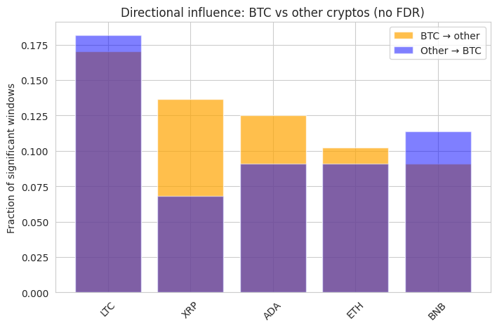
Source: Yahoo Finance
Interpretation of the plot:
Orange bars higher than blue bars → BTC dominates as a causal driver.
If some blue bars are comparable, it means reverse causality exists (maybe smaller altcoins occasionally influence BTC, e.g., during hype events).
import matplotlib.pyplot as plt

# Top 5 strongest BTC → other cryptos
top_n = 5
top_links = btc_cause_no_fdr.head(top_n)

plt.figure(figsize=(8,5))
plt.bar(top_links['effect'], top_links['frac_significant'], color='orange', alpha=0.8)
plt.ylabel('Fraction of significant windows')
plt.xlabel('Effect Cryptos')
plt.title(f'Top {top_n} BTC → other cryptos (strongest stable links)')
plt.ylim(0,1)
plt.grid(axis='y', linestyle='--', alpha=0.5)
for i, val in enumerate(top_links['frac_significant']):
    plt.text(i, val+0.02, f"{val:.2f}", ha='center', va='bottom', fontsize=10)
plt.show()
Source: Yahoo Finance
● This study examined causal linkages among six major cryptocurrencies (BTC, ETH, BNB, ADA, XRP, LTC) using the Toda–Yamamoto framework applied in rolling windows. The analysis highlights how inference is strongly shaped by the treatment of multiple testing.
● Raw (no-FDR) results suggest a dense network of apparent causal connections, with Bitcoin and Litecoin often emerging as influential senders. However, once false discovery rate (FDR) adjustments are applied, the network becomes far sparser: leadership effects are weak, intermittent, and often non-persistent. The contrast between pre-FDR and FDR-adjusted results underscores how easily raw significance can overstate structure when many tests are conducted simultaneously.
● The stability leaderboard (Table 3) shows that only a handful of relations display consistent significance across windows, and even these weaken under stricter corrections. LTC → BNB is the most robust under raw and per-window FDR settings, while ADA → XRP and XRP → ETH show local robustness. Under global FDR, only a few links such as BNB → LTC and BTC → XRP survive, emphasizing the rarity of truly persistent causal effects.
● Overall, our findings suggest that causal relations in crypto returns are weak, transient, and highly sensitive to multiple-testing adjustments. Claims of persistent dominance—such as Bitcoin being a universal driver—are not supported once proper corrections are applied. This highlights the importance of controlling for false discoveries in high-dimensional time-series causality analysis.
Information posted on IBKR Campus that is provided by third-parties does NOT constitute a recommendation that you should contract for the services of that third party. Third-party participants who contribute to IBKR Campus are independent of Interactive Brokers and Interactive Brokers does not make any representations or warranties concerning the services offered, their past or future performance, or the accuracy of the information provided by the third party. Past performance is no guarantee of future results.
This material is from Quant Insider and is being posted with its permission. The views expressed in this material are solely those of the author and/or Quant Insider and Interactive Brokers is not endorsing or recommending any investment or trading discussed in the material. This material is not and should not be construed as an offer to buy or sell any security. It should not be construed as research or investment advice or a recommendation to buy, sell or hold any security or commodity. This material does not and is not intended to take into account the particular financial conditions, investment objectives or requirements of individual customers. Before acting on this material, you should consider whether it is suitable for your particular circumstances and, as necessary, seek professional advice.
Trading in digital assets, including cryptocurrencies, is especially risky and is only for individuals with a high risk tolerance and the financial ability to sustain losses. Eligibility to trade in digital asset products may vary based on jurisdiction.
Please keep in mind that the examples discussed in this material are purely for technical demonstration purposes, and do not constitute trading advice. Also, it is important to remember that placing trades in a paper account is recommended before any live trading.


Join The Conversation
For specific platform feedback and suggestions, please submit it directly to our team using these instructions.
If you have an account-specific question or concern, please reach out to Client Services.
We encourage you to look through our FAQs before posting. Your question may already be covered!