Excel: VLOOKUP with a Vector of Lookup Values

The article “Excel: VLOOKUP with a Vector of Lookup Values” was originally posted on SHLee AI Financial Model.

This post presents an advanced Excel technique for the quadratic form matrix calculation accompanying cross products with correlation. This approach allows the user to change only input data and get the correct result without modifications of Excel formula.

Problem and Expected Output

Let  denotes the weighted sensitivities at maturities (M) in currencies (C). Our problem is to calculate which is the aggregation of these across maturities within each currency

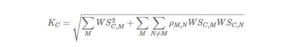
Here, M = {2w, 6w, …, 1Y, 2Y,…} and C = {USD, EUR, …}

This equation can be rewritten as the following quadratic form.

Here, m is the number of elements of M.

In other words, we can calculate element-by-element cross products with correlation or quadratic form matrix multiplication.

Before doing this job, we need to sort dataset by key columns such as currency code and maturity. Sorted input dataset and the expected output are as follows.

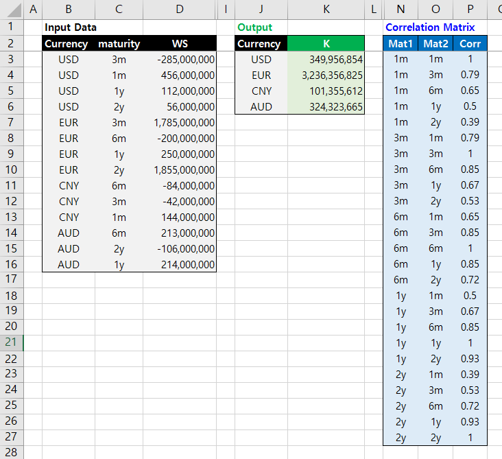
As can be seen in the above Excel information, our purpose is to calculate K within each currency from input data using the aforementioned quadratic (or cross product type) form formula with correlation matrix . The following figure is the our proposed Excel formula in the case of EUR.

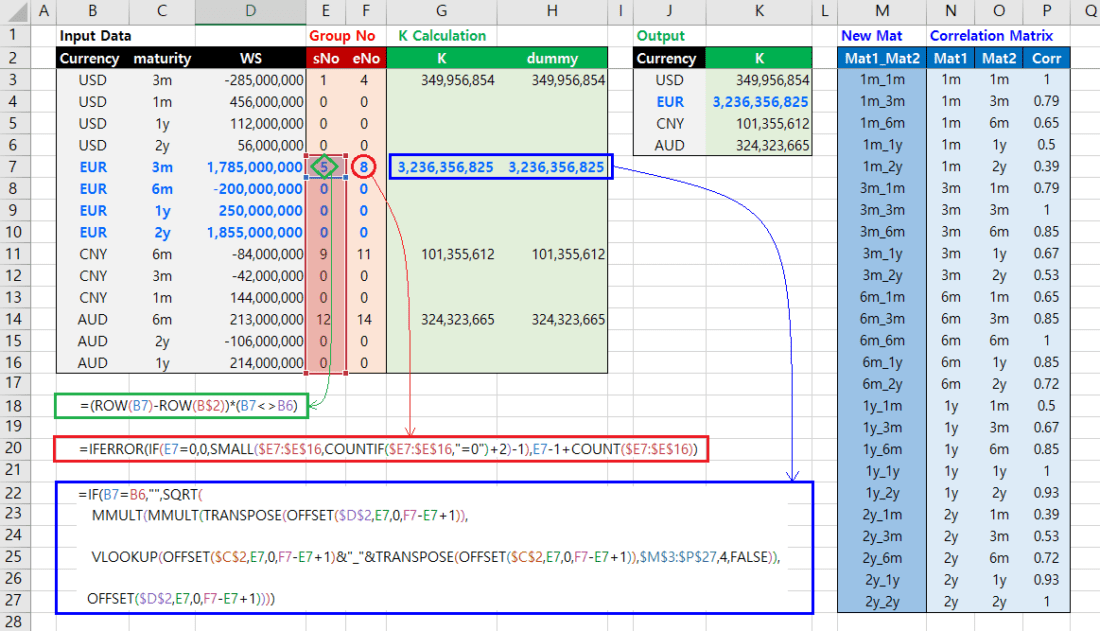
These set of Excel formula are explained as the following order.

1. get start and end row for each currency group
2. add composite maturity column to correlation information
3. calculate  by each currency group
4. collect non-empty cells for reporting

Determination of Start and End Row by Currency

For currency group operations, we split input data according to each currency. As such, we add two columns (sNo, eNo), which indicate relative number of start and end row for each currency from column name line (row = 2). Inserting and dragging two Excel formula generate sNo and eNo. For example, in the case of EUR, Excel formula for sNo and eNo have the following form.

"7E" <- (ROW(B7)-ROW(B$2))*(B7<>B6)
 
"7F" <- IFERROR(
        IF(E7=0,0,
              
           SMALL($E7:$E$16, COUNTIF($E7:$E$16,"=0")+2)-1),
              
        E7-1+COUNT($E7:$E$16)
      )

Add Concatenated Maturity to Correlation table

To find the correct correlation between two maturities (Mat1, Mat2) by using VLOOKUP() function, we need to make two input maturities into one input. We, therefore, add Mat1_Mat2 column which is the concatenation of Mat1 and Mat2 strings with underline(“_”) in between.

Calculation of Kc by Currency

This calculation is the main content of this post. We perform the abovementioned quadratic form matrix calculation. It is worth noting that as the first input argument of VLOOKUP function, we use not one string but a vector of strings (composite maturity code; Mat1_Mat2).

Calculation of  by currency code can be easily done by one vector operation with CTRL+SHIFT+ENTER and dragging.

But unlike our normal expectation, applying this operation with CTRL+SHIFT+ENTER to one cell results in “#VALUE!”. I think Excel has some error for this type of operation. Because we can’t modify Excel itself, we sidestep this problem and apply this operation with CTRL+SHIFT+ENTER to any two cells not one cell.

As we are all expected, it is correct for this operation is applied into one cell with subsequent dragging because output is one value per one currency. But Excel requires at least two cells for this vector operation with CTRL+SHIFT+ENTER. For this reason, I also include “Dummy” column for two-cell operation. Of course, when we use two cells, correct answer is returned and we have only to read value from the first cell not Dummy cell.

In short, at Row 3 in Excel spreadsheet, our vector operation with CTRL+SHIFT+ENTER is applied to G3:H3 (two cells) and apply this operation by dragging all rows.

=IF(B7=B6,"",SQRT(
MMULT(MMULT(TRANSPOSE(OFFSET($D$2,E7,0,F7-E7+1)),
 
VLOOKUP(OFFSET($C$2,E7,0,F7-E7+1)&"_"&TRANSPOSE(OFFSET($C$2,E7,0,F7-E7+1)),
               $M$3:$P$27, 4, FALSE)),
 
OFFSET($D$2,E7,0,F7-E7+1))))

At first, left row vector (LR) and right column vector (RC) are determined by using OFFSET() function with information of sRow and eRow for EUR.

LR : TRANSPOSE(OFFSET($D$2,E7,0,F7-E7+1))
RC :           OFFSET($D$2,E7,0,F7-E7+1)

There is the correlation matrix  between two vectors, which is constructed by using VLOOKUP() function. As a lookup value for VLOOKUP() function, string concatenation of two maturities with “_” are used and these maturities are also easily determined by using OFFSET() function with information of sRow and eRow for EUR.

CORR(rho) : 
 
VLOOKUP(OFFSET($C$2,E7,0,F7-E7+1)&"_"&
        TRANSPOSE(OFFSET($C$2,E7,0,F7-E7+1)),
        $M$3:$P$27,4,FALSE)),

A lookup value for VLOOKUP() function is known as one string or number. But as you can see from the above our Excel formula, a vector of lookup values are also used.

Collecting Non-empty Cells

Collecting non-empty cells is done by the following Excel formula for the K4 cell (EUR).

=IFERROR(
    INDEX($B$3:$G$16,
      SMALL( ($G$3:$G$16<>"")*(ROW($G$3:$G$16)-ROW($G$2)),
              COUNTBLANK($G$3:$G$16)+ROW($G4)-ROW($G$2) ),
      MATCH(K$2,$B$2:$G$2,0)
    ),"")

This is already explained in the previous post.

• Excel : Calculation by group and collecting non-empty cells

Benefit of This Excel Technique

Although input data is changed, we can get the correct results without any modification of Excel formula. This point is a merit of our approach. As Troy Olson said that if a picture is worth a thousand words, then a video is worth a million, Let’s see the following.

Changes of Input and the corresponding results

Visit SHLee AI Financial Model blog to watch the video on creating a VLOOKUP macro.

This advanced Excel technique will help reduce annoying jobs when input data is changed regularly or irregularly.