Refined academic research note (with charts, methodology, and references)

Data window: 2025-02-24 to 2026-02-20 • N=238 daily observations

Disclosure & limitations. This note is for educational/informational purposes. Results are computed from a single return series provided by the author and are not audited. Statistics are computed on daily returns with a zero risk‑free rate assumption unless stated otherwise; transaction costs, financing, slippage, taxes, and borrow costs are not included. Past performance is not indicative of future results.

Abstract

We evaluate an Equity Market Neutral (EMN) long/short portfolio against SPX using 238 daily observations from 2025‑02‑24 to 2026‑02‑20. Across the sample, EMN exhibits higher risk‑adjusted performance and lower drawdown than the equity benchmark. EMN achieves an annualized Sharpe ratio of 2.54 versus 0.83 for SPX, with cumulative returns of 42.8% versus 14.9%. Path and tail risk metrics are also favorable: EMN’s maximum drawdown is −6.0% versus −16.9% for SPX, and its historical 1‑day VaR95 is −1.27% versus −1.70%. At lower frequency, EMN wins 69.2% of weeks and 69.2% of months (SPX: 53.8% and 61.5%). Diagnostics show low market dependence (beta≈0.16, correlation≈0.21) and no statistically significant daily return autocorrelation over 20 lags.

1. Motivation and framing

Equity market neutral strategies are typically evaluated not primarily on raw returns, but on their ability to deliver diversifying, risk-efficient performance with limited dependence on equity market direction. This note therefore emphasizes (i) risk-adjusted performance (Sharpe, information ratio), (ii) downside and tail risk (drawdown, VaR and CVaR), and (iii) time-series diagnostics (autocorrelation and rolling behavior).

The specific hypothesis examined is that an EMN portfolio built from DEX-derived support/resistance levels and additional options-flow confirmation can produce (a) attractive risk-adjusted returns and (b) a smoother path than long-only equity exposure, while maintaining low beta to SPX.

Because performance metrics can be sensitive to sampling window, parameter choices, and market regimes, the results should be interpreted as a descriptive analysis of the provided period. The natural next step in a formal due diligence process would be multi-year analysis and out-of-sample validation.

2. EMN strategy overview (signal construction and portfolio rules)

The EMN portfolio is a systematic long/short equity strategy that combines (i) dealer-exposure-derived (DEX) support/resistance levels and (ii) signed options-flow information to select and size positions. The design goal is to reduce directional market exposure while extracting alpha from microstructure-linked flows and price-level effects.

2.1 Trade selection rules

Positions are selected and sized using the following rules:

1. Go long at DEX-defined support when options flows are net-positive.
2. Go short at DEX-defined resistance when options flows are net-negative.
3. Maintain 7 long positions and 7 short positions (14 gross names).
4. Apply volatility-based position sizing (lower volatility → larger notional; higher volatility → smaller notional) so that positions contribute more comparable ex ante risk.

Volatility-based sizing can be implemented in many ways. A common approach is inverse-volatility weighting:

    w_i ∝ 1 / σ̂_i

where σ̂_i is an estimate of recent realized volatility (e.g., 20–60 trading days). This targets a more uniform risk contribution across positions and helps prevent a small subset of high-volatility names from dominating portfolio risk. From a practical standpoint, volatility sizing also tends to ‘auto-delever’ during turbulence if volatility estimates react quickly.

“Managed portfolios that take less risk when volatility is high … increase Sharpe ratios.”

— Moreira & Muir (2017), Volatility‑Managed Portfolios

2.2 What “DEX-derived support/resistance” means in practice

DEX levels are derived from options positioning and the hedging mechanics of dealers/market makers. Large concentrations of options exposure at particular strikes can induce hedging flows that influence price dynamics as the underlying approaches those levels. When dealers are net long gamma, hedging flows can dampen price moves (range-like behavior); when dealers are net short gamma, hedging can amplify moves (trend/instability).

This mechanism has been studied in academic work linking dealer gamma imbalances to intraday momentum/reversal and volatility regimes. Although practitioners may compute DEX/GEX measures with different conventions (e.g., choice of maturities, dealer sign assumptions, or smoothing), the core intuition is consistent: delta-hedging flows are mechanical, and the sign of gamma changes the stabilizing vs destabilizing nature of those flows.

“We document a link between large aggregate dealers’ gamma imbalances and intraday momentum/reversal of stock returns.”

— Barbon & Buraschi (2021), Gamma Fragility

2.3 Why options flow is a complementary confirmatory signal

Options markets are not merely a derivative venue; they are a locus of informed trading and risk transfer. Signed options-flow measures attempt to capture the direction and intensity of demand for delta (directional exposure) or vega (volatility exposure). In EMN, these flows act as a confirmation filter: DEX supplies candidate levels; options flow supplies a directional/regime confirmation.

“Option volume contains information about the future direction of underlying stock price movements.”

— Pan & Poteshman (2006), referenced by Ni, Pan & Poteshman (2008)

2.4 Portfolio construction for market neutrality

“Market neutral” can mean different things operationally. Common implementations include dollar neutrality (equal long and short notional), beta neutrality (estimated beta to the market near zero), and/or sector neutrality (balanced exposures by sector). The 7-long/7-short structure primarily supports dollar neutrality and breadth. To the extent that names have heterogeneous betas, beta neutrality typically requires beta-aware weighting or constrained optimization.

Empirically, the realized beta of EMN vs SPX over the sample is low (≈0.16). This does not prove structural neutrality in all regimes—betas can rise in crises—but it is directionally consistent with the market-neutral objective.

3. Data and methodology

The dataset contains daily simple returns for EMN and SPX over 238 trading days from 2025-02-24 to 2026-02-20. Weekly returns are compounded from daily returns within a Friday-to-Friday week. Monthly returns are compounded within calendar months at month-end.

3.1 Estimation choices and conventions

Unless otherwise stated, the following conventions are used:

• Trading days per year: 252 (annualization factor).
• Risk-free rate: 0% (Sharpe is computed on raw returns). Over a one-year window, using a positive cash rate would reduce Sharpe slightly.
• VaR: historical (empirical) 5th percentile of daily returns.
• Max drawdown: computed on a $1 equity curve obtained by compounding returns.

3.2 Metric definitions and intuition

Sharpe ratio summarizes average return per unit of total volatility. It is a second-moment metric and therefore compresses the return distribution to mean and variance. Two practical issues arise: (i) fat tails and skew can make variance an incomplete risk descriptor, and (ii) serial correlation can bias standard errors and annualization.

Max drawdown captures path risk: the largest cumulative loss from a prior peak. Drawdown is particularly important for leveraged or capacity-constrained strategies, because a sufficiently deep drawdown can trigger forced deleveraging.

VaR summarizes a quantile of the loss distribution but is not subadditive and does not describe the magnitude of losses beyond the quantile. CVaR (expected shortfall) addresses this by averaging losses in the tail beyond VaR.

4. Empirical results (EMN vs SPX)

Table 1 summarizes the primary statistics computed directly from the supplied return series.

4.1 Risk-adjusted return: Sharpe ratio

EMN’s annualized Sharpe ratio (2.54) materially exceeds SPX’s (0.83). Under a simple mean-variance lens, this indicates that EMN delivered substantially more average daily return per unit of realized volatility.

However, Sharpe should not be interpreted as a complete risk measure. If returns are fat-tailed or negatively skewed, a high Sharpe can coexist with large tail losses. This note therefore pairs Sharpe with drawdown, VaR/CVaR, and distribution diagnostics (skewness and kurtosis).

4.2 Return compounding: cumulative return vs CAGR

Cumulative return measures total growth over the sample, while CAGR annualizes this growth geometrically. Over the sample, EMN’s cumulative return is 42.82% with a CAGR of 45.84%. SPX’s cumulative return is 14.92% with a CAGR of 15.86%. CAGR is especially relevant for allocators evaluating long-run compounding.

4.3 Path risk: drawdown and recovery

Maximum drawdown captures the worst capital impairment experienced during the sample. EMN’s max drawdown is −6.0% compared with −16.9% for SPX.

Drawdown matters because recovery is nonlinear. A drawdown of d requires a gain of d/(1−d) to recover. For example, a 6% drawdown requires ~6.4% gain to recover, while a 16.9% drawdown requires ~20.3% gain. Strategies with smaller drawdowns can therefore compound more efficiently even if average returns are similar.

4.4 Tail risk: VaR95 and CVaR95

EMN’s historical 1-day VaR95 is -1.27%, while SPX’s is -1.70%. Expected shortfall (CVaR95) is -1.75% for EMN and -3.01% for SPX. CVaR is more tail-sensitive because it averages outcomes beyond the VaR quantile.

“Conditional value‑at‑risk … has significant advantages over value‑at‑risk.”

— Rockafellar & Uryasev (2000/2002)

A practical interpretation is that VaR answers “how bad is a typical bad day,” while CVaR answers “how bad are the worst 5% of days on average.” For strategies exposed to gap risk or option-like payoff convexities, CVaR and stress tests are generally more informative than VaR alone.

4.5 Consistency: weekly and monthly win rates

EMN is positive in 69.2% of weeks and 69.2% of months. SPX is positive in 53.8% of weeks and 61.5% of months. Because win rate ignores magnitude, it is best interpreted together with tail metrics and distributional asymmetry.

4.6 Rolling 3-month returns and rolling risk

Rolling quarterly returns help reveal whether performance is concentrated in a single short episode or distributed across sub-periods. Rolling volatility and rolling Sharpe provide diagnostics on whether returns were achieved by taking time-varying risk or by maintaining stable risk through time.

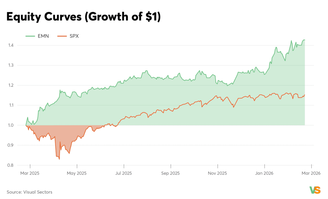
Figure 1. Equity curves (growth of $1).

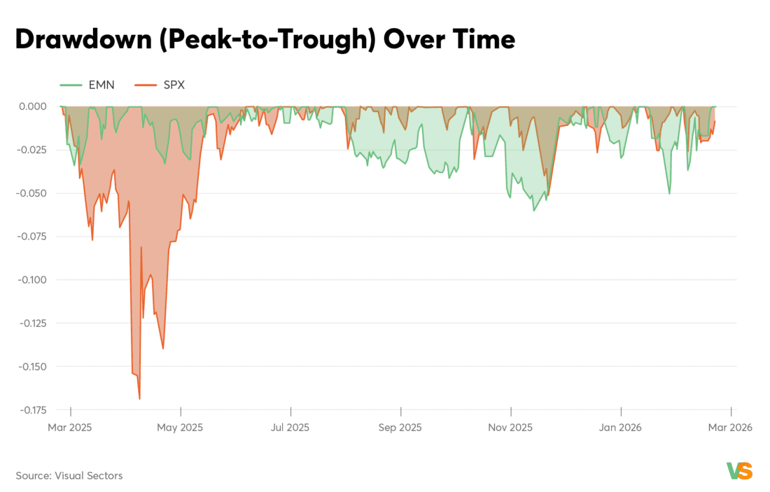
Figure 2. Drawdown paths (peak-to-trough over time).

Figure 3. Rolling 3-month compounded returns (month-end).

Figure 4A. Rolling 3-month return heatmap (EMN, by ending month).

Figure 4B. Rolling 3-month return heatmap (SPX, by ending month).

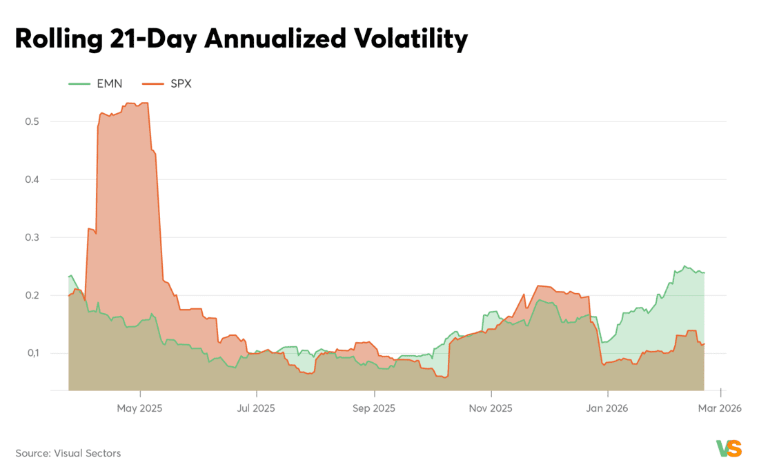
Figure 5. Rolling 21-day annualized volatility (risk regime).

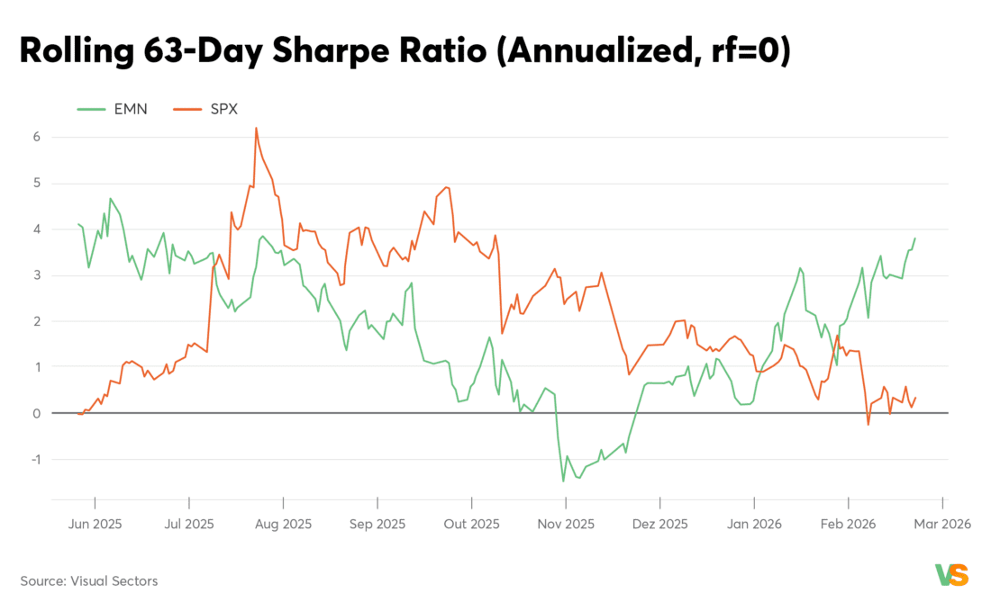
Figure 6. Rolling 63-day Sharpe ratio (annualized, rf=0).

Table 2 reports additional distribution and downside-risk statistics (computed from the same return series).

5. Benchmark-relative behavior: beta, correlation, and information ratio

Market-neutral strategies are often assessed by (i) how much market exposure they carry and (ii) how efficiently they generate active returns. We estimate beta and correlation of EMN to SPX on daily returns, and compute the information ratio of EMN relative to SPX.

Estimated beta (EMN vs SPX) is 0.16 and correlation is 0.21. Active returns (EMN − SPX) exhibit an annualized tracking error of 22.66%, an annualized active (geometric) growth rate of 21.68%, and an information ratio of 0.98.

Interpretation: low beta reduces vulnerability to broad market selloffs; the information ratio translates this into an efficiency metric—active return per unit of active risk.

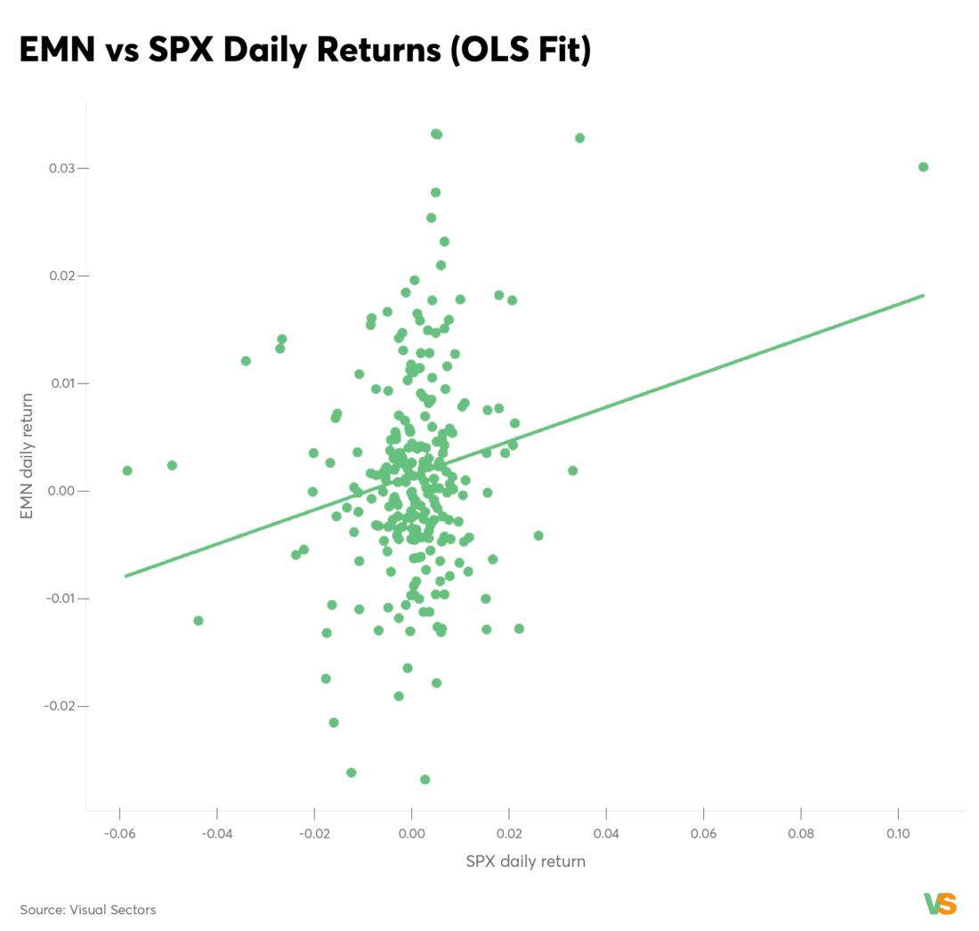
Figure 7. EMN vs SPX daily returns with OLS fit.

Figure 8. Active return (EMN − SPX): growth of $1.

Figure 9. Rolling information ratio of active returns (63 trading day window).

6. Statistical diagnostics: autocorrelation and return structure

Serial correlation in returns can indicate regime persistence, microstructure effects, or return smoothing. We analyze the autocorrelation function (ACF) up to 20 lags and perform Ljung–Box tests for joint significance.

EMN: no statistically significant autocorrelation is detected (Ljung–Box p‑values: 0.810 at lag 10; 0.848 at lag 20). SPX: autocorrelation is statistically significant over the same horizon (p‑values: 0.002 at lag 10; 0.004 at lag 20).

One interpretation is that SPX exhibits short-horizon mean reversion and volatility clustering, which can generate statistically detectable autocorrelation at daily lags. In EMN, the absence of significant autocorrelation is consistent with a return stream driven by many idiosyncratic moves that do not mechanically repeat day-to-day.

For risk estimation, this matters because serial correlation can bias naïve annualization and understate true uncertainty. Allocators often complement these diagnostics with block bootstrap methods or Newey–West standard errors when formal inference is required.

Figure 10. Autocorrelation of daily returns (ACF) with 95% confidence band.

7. Market-neutral construction and win rate amplification

At the single-name level, signals often have modest directional accuracy (hit rate slightly above 50%). Portfolio construction can amplify this into a more stable return stream by reducing variance contributed by market direction and idiosyncratic noise.

The author reports a 52.91% hit rate at the individual-name level for the underlying selection process. In this sample, EMN’s weekly win rate is 69.2%. While the horizons are not identical, the direction is consistent with the hypothesis that market neutrality and diversification improve consistency.

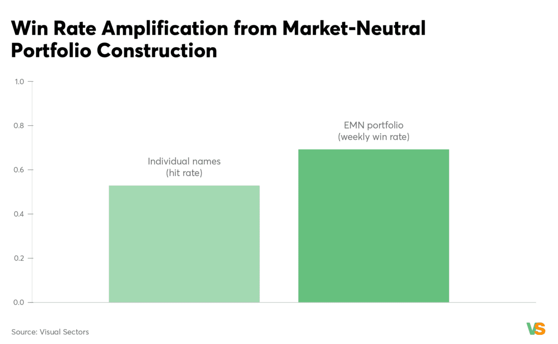
Figure 11. Win rate amplification: individual-name hit rate (reported) vs EMN portfolio weekly win rate (observed).

7.1 A factor-model explanation

Under a simple factor model, a stock’s return can be decomposed into market and idiosyncratic components. If the portfolio is constructed to target near-zero beta, then the market component is reduced, shrinking return variance without necessarily shrinking expected alpha. Because win probability for a given horizon increases with the mean-to-variance ratio, this can raise observed win rates at weekly and monthly frequencies.

7.2 Breadth and the information ratio

The fundamental law of active management provides intuition for why breadth matters: risk-adjusted performance increases with both forecasting skill and breadth (the number of independent bets). A 7-long/7-short structure increases breadth relative to single-name trading and can mitigate concentration risk. This is not a free lunch—correlations can spike in crises—but it is a core mechanism behind market-neutral portfolio construction.

8. Proprietary data as edge in the AI era

Modern toolchains (including large language models) reduce the cost of generating strategies from public price/volume features (moving averages, oscillators, breakouts, and other standard technical indicators). As a result, sustainable edge often shifts from implementation to information: unique datasets, superior labeling, and better microstructure understanding.

Empirical evidence suggests that widely disseminated predictors can attenuate as arbitrage capital learns and trades them. McLean and Pontiff document meaningful post-publication decay in return predictability, consistent with crowding in public signals. Related work on quant crowding emphasizes that when many investors hold similar trades, returns can compress and crash risk can rise.

“Portfolio returns are 26% lower out‑of‑sample and 58% lower post‑publication.”

— McLean & Pontiff (2016)

Options-flow and dealer-positioning measures are not simple functions of OHLC; they require specialized data and interpretation. Academic evidence supports their relevance: option volume and demand contain information about future stock price direction and volatility, and dealer gamma positioning can influence intraday momentum/reversal and volatility regimes. Taken together, this literature supports the claim that proprietary options-derived datasets can contain incremental information beyond OHLC.

8.1 Practical implications for research and execution

In practice, building a durable edge around these signals requires:

• Robust trade classification for options flow (buyer- vs seller-initiated).
• Consistent aggregation of delta/gamma exposure across strikes and maturities.
• Careful handling of corporate actions and symbol changes.
• Realistic execution modeling (bid/ask, market impact, borrow availability).

These steps are difficult to commoditize and often determine whether a signal survives live deployment.

9. Limitations and next tests

This note evaluates one return series over roughly one year. A thorough investment due diligence process would typically require:

• Multi-year evaluation across materially different volatility regimes, including crisis episodes.
• Transaction cost modeling (commissions, slippage, borrow costs, financing).
• Capacity analysis and liquidity stress tests.
• Exposure attribution to ensure returns are not an unintended bet on standard equity factors.
• Robustness checks to parameter choices (DEX construction, flow windows, volatility estimators) and to estimation error.

Appendix A. Metric formulas and implementation notes

A.1 Sharpe ratio (annualized, rf=0)

Sharpe = (mean(r_d) / std(r_d)) × √252, where r_d are daily returns.

A.2 Cumulative return and CAGR

Cumulative = ∏(1 + r_d) − 1. CAGR = (∏(1+r_d))^(252/N) − 1.

A.3 Max drawdown

Equity_t = ∏_{s≤t}(1+r_s). Drawdown_t = Equity_t / max_{u≤t}(Equity_u) − 1. MaxDD = min(Drawdown_t).

A.4 Historical VaR95 and CVaR95

VaR95 is the empirical 5th percentile of daily returns. CVaR95 is the mean of returns less than or equal to VaR95.

A.5 Information ratio

Active_t = r_EMN,t − r_SPX,t. IR = (mean(Active) / std(Active)) × √252.

A.6 Weekly/monthly returns and win rate

Weekly return: ∏(1+r_d)−1 within each week (Fri close). Win rate: fraction of weeks with return > 0. Monthly analog at month-end.

A.7 Autocorrelation and Ljung–Box

ACF(k) = corr(r_t, r_{t−k}). Ljung–Box tests joint significance of ACFs up to a chosen lag.

Appendix B. Distribution diagnostics

Return distributions are non-normal in this sample (Jarque–Bera rejects normality for both EMN and SPX), which motivates non-parametric tail metrics and stress testing beyond Gaussian assumptions.

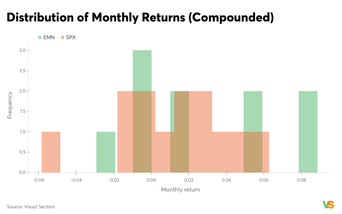
Figure 13. Monthly return distributions (histograms).

Appendix C. Reproducibility notes

All charts and statistics in this note are computed directly from the provided daily return series. Annualization uses a 252 trading-day convention. Weekly returns compound daily returns into Friday weeks; monthly returns compound to month-end. VaR and CVaR are computed historically from the empirical daily return distribution.

References (linked)

Moreira, A., & Muir, T. (2017). Volatility-Managed Portfolios. Journal of Finance.

Rockafellar, R. T., & Uryasev, S. (2000/2002). Conditional Value-at-Risk for General Loss Distributions.

Pan, J., & Poteshman, A. M. (2006). The Information in Option Volume for Future Stock Prices.

Ni, S. X., Pan, J., & Poteshman, A. M. (2008). Volatility Information Trading in the Option Market.

Gârleanu, N., Pedersen, L. H., & Poteshman, A. M. (2005/2009). Demand-Based Option Pricing.

Barbon, A., & Buraschi, A. (2021). Gamma Fragility.

Baltussen, G., Da, Z., Lammers, D., & Martens, M. (2021). Hedging Demand and Market Intraday Momentum.

Lo, A. W., Mamaysky, H., & Wang, J. (2000). Foundations of Technical Analysis. Journal of Finance (NBER WP 7613).

McLean, R. D., & Pontiff, J. (2016). Does Academic Research Destroy Stock Return Predictability? (working paper version).

Cahan, R., & Luo, Y. (2013). Measuring Crowding in Quantitative Strategies.