Delta Sensitivity of Interest Rate Swap

This post explains how to calculate delta sensitivities or delta vector of interest rate swap. Delta can be calculated by either 1) zero delta or 2) market delta. To the best of our knowledge, FRTB can use these two methods but SIMM use the market Greeks. We implement R code for two approaches.

Introduction

For detailed information about the Libor IRS swap pricing and zero curve bootstrapping, refer to the following posts.

In previous posts, we have priced a 5Y Libor IRS swap and generated a zero curve from market swap rates by using bootstrapping. Based on these works, we calculate Greeks of IRS. Since IRS does not have any option characteristics, our focus is to calculate the delta sensitivities or delta vector. And for convenience, swap value is defined as (floating leg – fixed leg).

Delta Sensitivity

ISDA SIMM uses the following definitions of interest rate risk delta (xx is a risk factor). There are, of course, several versions of it but they are all essentially the same.

For ease of notation, let z(t) and s(t) denote the (bootstrapped) zero rates or zero curve and (market observed) swap rates or swap curve at time t respectively.

There are two approaches for the calculation of delta: 1) zero delta, 2) market delta.

Zero Delta

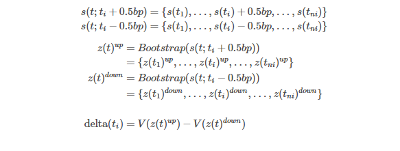
Zero delta approach calculates delta sensitivities by bumping up or down zero rates one by one in order.

Once the zero curve (z(t)) is generated from market swap rates (s(t)),

Bumping up (z(t_; t_i + 0.5bp) or down (z(t_; t_i−0.5bp)), delta(t_i) is calculated and this process is applied for all t_i.

Here, t_i, i = 1, 2,…, n_i = 1, 2,…, n _i are maturities or dates of market swap rates at which the corresponding zero rates are bootstrapped.

Market Delta

Market delta approach calculates delta sensitivities by bumping up or down market swap rates one by one in order. Unlike the zero delta, every time we bump one market swap rate of a selected maturity, we should run a bootstrapping for finding new zero curve. Using this newly generated zero curve, we can calculate delta sensitivity at time t_i as follows.

The following R code calculates delta sensitivities of IRS using these two approaches.

#=========================================================================#
# Financial Econometrics & Derivatives, ML/DL using R, Python, Tensorflow  
# by Sang-Heon Lee 
#
# https://kiandlee.blogspot.com
#————————————————————————-#
# Calculate Delta Sensitivities of Libor IRS
#=========================================================================#
 
graphics.off()  # clear all graphs
rm(list = ls()) # remove all files from your workspace
 
#=========================================================================
# Functions – Definition
#=========================================================================
 
#————————————————————–
# Calculation of IRS swap price
#————————————————————–
f_zero_prr_IRS <– function(
    fixed_rate,                   # fixed rate
    vd.fixed_date, vd.float_date, # date for two legs
    vd.zero_date,  v.zero_rate,   # zero curve (dates, rates)
    d.spot_date,   no_amt,        # spot date, nominal amt
    save_cf_yn) {                 # “y” : CF save                     
 
    #———————————————————-
    # 0) Preprocessing
    #———————————————————-
    
    # convert spot date from date(d) to numeric(n)
    n.spot_date <– as.numeric(d.spot_date)
    
    # Interpolation of zero curve
    vn.zero_date <– as.numeric(vd.zero_date)
    f_linear     <– approxfun(vn.zero_date, v.zero_rate, 
                          method=“linear”)
    vn.zero_date.inter <– n.spot_date:max(vn.zero_date)
    v.zero_rate.inter  <– f_linear(vn.zero_date)
    
    # number of CFs
    ni <– length(vd.fixed_date)
    nj <– length(vd.float_date)
    
    # output data.frame with CF dates and its interpolated zero
    df.fixed = data.frame(d.date = vd.fixed_date,
                          n.date = as.numeric(vd.fixed_date))
    df.float = data.frame(d.date = vd.float_date,
                          n.date = as.numeric(vd.float_date))
    
    #———————————————————-
    #  1)  Fixed Leg
    #———————————————————-
    
    # zero rate for discounting
    df.fixed$zero_DC = f_linear(as.numeric(df.fixed$d.date))
    
    # discount factor
    df.fixed$DF <– exp(–df.fixed$zero_DC*
                       (df.fixed$n.date–n.spot_date)/365)
    
    # tau, CF
    for(i in 1:ni) {
        
        ymd      <– df.fixed$d.date[i]
        ymd_prev <– df.fixed$d.date[i–1]
        if(i==1) ymd_prev <– d.spot_date
        
        d <– as.numeric(strftime(ymd, format = “%d”))
        m <– as.numeric(strftime(ymd, format = “%m”))
        y <– as.numeric(strftime(ymd, format = “%Y”))
        
        d_prev <– as.numeric(strftime(ymd_prev, format = “%d”))
        m_prev <– as.numeric(strftime(ymd_prev, format = “%m”))
        y_prev <– as.numeric(strftime(ymd_prev, format = “%Y”))
        
        # 30I/360
        tau <– (360*(y–y_prev) + 30*(m–m_prev) + (d–d_prev))/360
        
        # cash flow rate
        df.fixed$rate[i] <– fixed_rate
        
        # Cash flow at time ti
        df.fixed$CF[i] <– fixed_rate*tau*no_amt # day fraction
    }
    
    # Present value of CF
    df.fixed$PV = df.fixed$CF*df.fixed$DF
    
    
    #———————————————————-
    #  2)  Floating Leg
    #———————————————————-
    
    # zero rate for discounting
    df.float$zero_DC = f_linear(as.numeric(df.float$d.date))
    
    # discount factor
    df.float$DF <– exp(–df.float$zero_DC*
                       (df.float$n.date–n.spot_date)/365)
    
    # tau, forward rate, CF
    for(i in 1:nj) {
        
        date      <– df.float$n.date[i]
        date_prev <– df.float$n.date[i–1]
        
        DF        <– df.float$DF[i]
        DF_prev   <– df.float$DF[i–1]
        
        if(i==1) {
            date_prev <– n.spot_date
            DF_prev   <– 1
        }
        
        # ACT/360
        tau <– (date – date_prev)/360
        
        # forward rate
        fwd_rate <– (1/tau)*(DF_prev/DF–1)
        
        # cash flow rate
        df.float$rate[i] <– fwd_rate
        
        # Cash flow amount at time ti
        df.float$CF[i] <– fwd_rate*tau*no_amt # day fraction
    }
    
    # Present value of CF
    df.float$PV = df.float$CF*df.float$DF
    
    # check for cash flows
    if (save_cf_yn == “y”) {
        # print(df.float); print(df.fixed)
        write.csv(df.float, “CF_float.csv”)
        write.csv(df.fixed, “CF_fixed.csv”)
    }
 
    return(sum(df.float$PV) – sum(df.fixed$PV))
}
 
 
#————————————————————–
# IRS swap zero curve generator
#————————————————————–
f_zero_maker_IRS <– function(
    df.mt,                    # market information data.frame
                              # [d.date, swap_rate, source]]
    v.unknown_swap_maty_all,  # all unknown swap maturity
    vd.fixed_date,            # date for fixed leg
    vd.float_date,            # date for float leg
    d.spot_date,              # spot date
    no_amt) {                 # nominal principal amount
    
    # convert spot date from date(d) to numeric(n)
    n.spot_date <– as.numeric(d.spot_date)
    
    # for bootstrapped zero curve
    df.zr <– data.frame(
        d.date    = df.mt$d.date,
        n.date    = as.numeric(df.mt$d.date),
        tau       = as.numeric(df.mt$d.date) – n.spot_date,
        taui      = as.numeric(df.mt$d.date) – n.spot_date,
        swap_rate = df.mt$swap_rate, 
        zero_rate = rep(0,length(df.mt$d.date)),
        DF        = rep(0,length(df.mt$d.date)))
    
    # tau(i) = t(i) – t(i-1)
    df.zr$taui[2:nrow(df.zr)] <– 
        df.zr$n.date[2:nrow(df.zr)] – 
        df.# semi-annual date[1: (nrow(df.zr)–1)]
    
    # divide rows according to its source or instrument type
    rows_deposit <– which(df.mt$source==“deposit”)
    rows_futures <– which(df.mt$source==“futures”)
    rows_swap    <– which(df.mt$source==“swap”)
    
    #————————————————————–
    # 3. Bootstrapping – Deposit
    #————————————————————–
    
    for(i in rows_deposit) {
        
        # 1) calculate discount factor for deposit
        df.zr$DF[i] <– 1/(1+df.zr$swap_rate[i]*df.zr$tau[i]/360)
        
        # 2) convert DF to spot rate
        df.zr$zero_rate[i] <– 365/df.zr$tau[i]*log(1/df.zr$DF[i])
    }
    
    #————————————————————–
    # 4. Bootstrapping – Futures
    #————————————————————–
    
    # No convexity adjustment is made
    for(i in rows_futures) {
        
        # 1) discount factor from t(i-1) to t(i)
        df.zr$DF[i] <– 1/(1+df.zr$swap_rate[i]*df.zr$taui[i]/360)
        
        # 2) discount factor from spot date to t(i)
        df.zr$DF[i] <– df.zr$DF[i–1]*df.zr$DF[i]
        
        # 3) zero rate from discount factor
        df.zr$zero_rate[i] <– 365/df.zr$tau[i]*log(1/df.zr$DF[i])
    }
    
    #————————————————————–
    # 5. Bootstrapping – Swaps
    #————————————————————–
    
    k <– 1
    for(i in rows_swap) {
        
        # unknown swap maturity in year
        swap_maty <– v.unknown_swap_maty_all[k]
        
        # 1) find one unknown zero rate for one swap maturity
        m<–optim(0.01, objf,
            control = list(abstol=10^(–20), reltol=10^(–20),
                           maxit=50000, trace=2),
            method = c(“Brent”),
            lower = 0, upper = 0.1,               # for Brent
            v.unknown_swap_maty = swap_maty,      # unknown zero maturity
            v.swap_rate = df.zr$swap_rate[i],     # observed swap rate
            vd.fixed_date = vd.fixed_date,        # date for fixed leg
            vd.float_date = vd.float_date,        # date for float leg
            vd.zero_date_all = df.zr$d.date[1:i], # all dates for zero curve
            v.zero_rate_known  = df.zr$zero_rate[1: (i–1)], # known zero rates
            d.spot_date = d.spot_date, 
            no_amt = no_amt)
        
        # 2) update this zero curve with the newly found zero rate
        df.zr$zero_rate[i] <– m$par
        
        # 3) convert this new zero rate to discount factor
        df.zr$DF[i] <– exp(–df.zr$zero_rate[i]*df.zr$tau[i]/365)
        
        k <– k + 1
    }
    return(df.zr)
}
 
#————————————————————–
# objective function to be minimized
#————————————————————–
objf <– function(
    v.unknown_swap_zero_rate, # unknown zero curve (rates)
    v.unknown_swap_maty,      # unknown swap maturity
    v.swap_rate,              # fixed rate
    vd.fixed_date,            # date for fixed leg
    vd.float_date,            # date for float leg
    vd.zero_date_all,         # all dates for zero curve
    v.zero_rate_known,        # known zero curve (rates)
    d.spot_date,              # spot date
    no_amt) {                 # nominal principal amount
 
    # zero curve augmented with zero rates for swaps
    v.zero_rate_all <– c(v.zero_rate_known,
                         v.unknown_swap_zero_rate)
    
    v.swap_pr <– NULL # vector of swap prices
    
    k <– 1
    for(i in v.unknown_swap_maty) {
        
        # calculate IRS swap price
        swap_pr <– f_zero_prr_IRS(
            v.swap_rate[k],          # fixed rate, 
            vd.fixed_date[1: (2*i)],  # semi-annual date
            vd.float_date[1: (4*i)],  # quarterly   date
            vd.zero_date_all,        # zero curve (dates)
            v.zero_rate_all,         # zero curve (rates)
            d.spot_date, no_amt, “n”)
        
        # concatenate swap prices
        v.swap_pr <– c(v.swap_pr, swap_pr)
        k <– k + 1
    }
    
    return(sum(v.swap_pr^2))
}
 
#=========================================================================
# Main 
#=========================================================================
 
#————————————————————–
# 1. Market Information
#————————————————————–
 
# Zero curve from Bloomberg as of 2021-06-30 until 5-year maturity
df.mt <– data.frame(
    
    d.date = as.Date(c(“2021-10-04”,“2021-12-15”,
                       “2022-03-16”,“2022-06-15”,
                       “2022-09-21”,“2022-12-21”,
                       “2023-03-15”,“2023-07-03”,
                       “2024-07-02”,“2025-07-02”,
                       “2026-07-02”)),
    
    # we use swap rate not zero rate.
    swap_rate= c(0.00145750000000000,
                 0.00139609870272047,
                 0.00203838571440434,
                 0.00197747863867587,
                 0.00266249271921742,
                 0.00359490949297661,
                 0.00512603194652204,
                 0.00328354999423027,
                 0.00571049988269806,
                 0.00793000012636185,
                 0.00964949995279312
    ),
 
    source = c(“deposit”, rep(“futures”,6), rep(“swap”, 4))
)
 
#————————————————————–
# 2. Libor Swap Specification
#————————————————————–
 
d.spot_date  <– as.Date(“2021-07-02”)    # spot date (date type)
n.spot_date  <– as.numeric(d.spot_date)  # spot date (numeric type)
 
no_amt     <– 10000000      # notional principal amount
 
# swap cash flow schedule from Bloomberg 
lt.cf_date <– list( 
    
    fixed = as.Date(c(“2022-01-04”,“2022-07-05”,
                      “2023-01-03”,“2023-07-03”,
                      “2024-01-02”,“2024-07-02”,
                      “2025-01-02”,“2025-07-02”,
                      “2026-01-02”,“2026-07-02”)),
    
    float = as.Date(c(“2021-10-04”,“2022-01-04”,
                      “2022-04-04”,“2022-07-05”,
                      “2022-10-03”,“2023-01-03”,
                      “2023-04-03”,“2023-07-03”,
                      “2023-10-02”,“2024-01-02”,
                      “2024-04-02”,“2024-07-02”,
                      “2024-10-02”,“2025-01-02”,
                      “2025-04-02”,“2025-07-02”,
                      “2025-10-02”,“2026-01-02”,
                      “2026-04-02”,“2026-07-02”))
)
 
 
#————————————————————–
# 3. 5-year swap price : base
#————————————————————–
 
i = 5 # 5-year swap
 
# zero pricing
df.zr <– f_zero_maker_IRS(
           df.mt, c(2,3,4,5),
           lt.cf_date$fixed, lt.cf_date$float, 
           d.spot_date, no_amt)
 
pr    <– f_zero_prr_IRS(
           df.mt$swap_rate[i+6],
           lt.cf_date$fixed[1: (2*i)], 
           lt.cf_date$float[1: (4*i)],
           df.zr$d.date, df.zr$zero_rate, 
           d.spot_date,no_amt, save_cf_yn = “y”)
 
print(paste0(i,“-year Swap price at spot date = “, pr))
 
df.zr_delta    <– df.mt_delta    <– df.zr[,–c(2,3,4)]
df.zr_delta$pr <– df.mt_delta$pr <– pr
    
#————————————————————–
# 3. Bump and Reprice for Market Greeks
#————————————————————–
 
df.mt_delta$delta <– df.mt_delta$pr_up <– df.mt_delta$pr_dn <– NA
 
# iteration for all market maturities
for(r in 1:11) {
    
    #———————
    # bump up (1bp up)
    #———————
    df.mt_bump <– df.mt   # initialization
    df.mt_bump$swap_rate[r] <– df.mt_bump$swap_rate[r] + 0.0001 
    
    # zero pricing
    df.zr <– f_zero_maker_IRS(df.mt_bump, c(2,3,4,5),
               lt.cf_date$fixed, lt.cf_date$float, 
               d.spot_date, no_amt)
    pr    <– f_zero_prr_IRS(df.mt$swap_rate[i+6],
               lt.cf_date$fixed[1: (2*i)], 
               lt.cf_date$float[1: (4*i)],
               df.zr$d.date, df.zr$zero_rate, 
               d.spot_date, no_amt, “n”)
    
    # save price with bumping up
    df.mt_delta$pr_up[r] <– pr
    
    # check whether swap prices at spot date is at par
    pr    <– f_zero_prr_IRS(df.mt_bump$swap_rate[i+6],
               lt.cf_date$fixed[1: (2*i)],
               lt.cf_date$float[1: (4*i)],
               df.zr$d.date, df.zr$zero_rate, 
               d.spot_date,no_amt, “n”)
    
    print(paste0(i,“-year Swap price at spot date = “, pr))
    
    #———————
    # bump down (1bp down)
    #———————
    df.mt_bump <– df.mt   # initialization
    df.mt_bump$swap_rate[r] <– df.mt_bump$swap_rate[r] – 0.0001 
    
    # zero pricing
    df.zr <– f_zero_maker_IRS(df.mt_bump, c(2,3,4,5),
               lt.cf_date$fixed, lt.cf_date$float, 
               d.spot_date, no_amt)
    
    pr <– f_zero_prr_IRS(df.mt$swap_rate[i+6],
            lt.cf_date$fixed[1: (2*i)], lt.cf_date$float[1: (4*i)],
            df.zr$d.date, df.zr$zero_rate, d.spot_date,no_amt, “n”)
    
    # save price with bumping down
    df.mt_delta$pr_dn[r] <– pr
    
    # check whether swap prict at spot date is at par
    pr <– f_zero_prr_IRS(df.mt_bump$swap_rate[i+6],
            lt.cf_date$fixed[1: (2*i)], lt.cf_date$float[1: (4*i)],
            df.zr$d.date, df.zr$zero_rate, d.spot_date,no_amt, “n”)
    
    print(paste0(i,“-year Swap price at spot date = “, pr))
}
 
# Market Greeks : Delta calculation
df.mt_delta$delta <– (df.mt_delta$pr_up – 
                      df.mt_delta$pr_dn)/2 
 
df.mt_delta
 
x11(width = 5, height = 3.5)
barplot(delta ~ substr(d.date,1,7), data = df.mt_delta, 
        width = 0.5, col = “blue”)
 
x11(width = 5, height = 3.5)
barplot(delta ~ substr(d.date,1,7), data = df.mt_delta[1:10,],
        width = 0.5, col = “green”)
 
 
 
#————————————————————–
# 4. Bump and Reprice for Zero Greeks
#————————————————————–
 
df.zr_delta$delta <– df.zr_delta$pr_up <– df.zr_delta$pr_dn <– NA
 
# zero pricing
df.zr <– f_zero_maker_IRS(df.mt, c(2,3,4,5),
                            lt.cf_date$fixed, lt.cf_date$float, d.spot_date, no_amt)
 
for(r in 1:11) {
 
    #———————
    # bump up (1bp up)
    #———————
    df.zr_bump    <– df.zr  # initialization
    df.zr_bump$zero_rate[r] <– df.zr_bump$zero_rate[r] + 0.0001
 
    # zero pricing
    pr   <– f_zero_prr_IRS(df.mt$swap_rate[i+6],
              lt.cf_date$fixed[1: (2*i)], lt.cf_date$float[1: (4*i)],
              df.zr_bump$d.date, df.zr_bump$zero_rate, 
              d.spot_date, no_amt, “n”)
    
    # save price with bumping up
    df.zr_delta$pr_up[r] <– pr
 
    #———————
    # bump down (1bp down)
    #———————
    df.zr_bump    <– df.zr  # initialization
    df.zr_bump$zero_rate[r] <– df.zr_bump$zero_rate[r] – 0.0001
 
    # zero pricing
    pr <– f_zero_prr_IRS(df.mt$swap_rate[i+6],
            lt.cf_date$fixed[1: (2*i)], lt.cf_date$float[1: (4*i)],
            df.zr_bump$d.date, df.zr_bump$zero_rate, 
            d.spot_date,no_amt, “n”)
    
    # save price with bumping down
    df.zr_delta$pr_dn[r] <– pr
}
 
# Market Greeks : Delta calculation
df.zr_delta$delta <– (df.zr_delta$pr_up – 
                      df.zr_delta$pr_dn)/2
 
df.zr_delta
 
x11(width = 5, height = 3.5)
barplot(delta ~ substr(d.date,1,7), data = df.zr_delta, 
        width = 0.5, col = “blue”)
 
x11(width = 5, height = 3.5)
barplot(delta ~ substr(d.date,1,7), data = df.zr_delta[1:10,],
        width = 0.5, col = “green”)
 
Colored by Color Scripter

Stay tuned for the next installment to learn about the output demonstrating zero delta vector along the maturities.

For additional insight on this topic and to download the R scripts, visit https://kiandlee.blogspot.com/2021/07/delta-sensitivity-of-interest-rate-swap.html.

Join The Conversation

For specific platform feedback and suggestions, please submit it directly to our team using these instructions.

If you have an account-specific question or concern, please reach out to Client Services.

We encourage you to look through our FAQs before posting. Your question may already be covered!

Visit IBKR.com Open an IBKR Account

Disclosure: Interactive Brokers Third Party

Information posted on IBKR Campus that is provided by third-parties does NOT constitute a recommendation that you should contract for the services of that third party. Third-party participants who contribute to IBKR Campus are independent of Interactive Brokers and Interactive Brokers does not make any representations or warranties concerning the services offered, their past or future performance, or the accuracy of the information provided by the third party. Past performance is no guarantee of future results.

This material is from SHLee AI Financial Model and is being posted with its permission. The views expressed in this material are solely those of the author and/or SHLee AI Financial Model and Interactive Brokers is not endorsing or recommending any investment or trading discussed in the material. This material is not and should not be construed as an offer to buy or sell any security. It should not be construed as research or investment advice or a recommendation to buy, sell or hold any security or commodity. This material does not and is not intended to take into account the particular financial conditions, investment objectives or requirements of individual customers. Before acting on this material, you should consider whether it is suitable for your particular circumstances and, as necessary, seek professional advice.

How much could you save on your margin loan by switching to Interactive Brokers?

Fill out the information below to see your estimated savings.

Current Interest Rate

Balance

USD

Margin Amount Borrowed

USD

Time Margin is Borrowed

IBKR will assess a surcharge of 1% on large loan balances unless otherwise prearranged with IBKR. The 1% surcharge would apply to all balances in the highest tier.

The interest calculator is based on information that we believe to be accurate and correct, but neither Interactive Brokers LLC nor its affiliates warrant its accuracy or adequacy and it should not be relied upon as such. Neither IBKR nor its affiliates are responsible for any errors or omissions or for results obtained from the use of this calculator.

Restrictions apply. Annual Percentage Rate (APR) on USD margin loan balances for IBKR Pro as of October 3, 2024. Interactive Brokers calculates the interest charged on margin loans using the applicable rates for each interest rate tier listed on its website. Learn more about margin loan rates.

The projections or other information generated by the Interest Calculator tool are hypothetical in nature, do not reflect actual results and are not guarantees of future results. Please note that results may vary with use of the tool over time.

Trading on margin is only for experienced investors with high risk tolerance. You may lose more than your initial investment. For additional information about rates on margin loans, please see Margin Loan Rates.

Master options fundamentals with our new Interactive Learning course