Building Blocks of Bias-Variance Tradeoff for Trading the Financial Markets

The article “Building Blocks of Bias-Variance Tradeoff for Trading the Financial Markets” was originally published on QuantInsti blog.

Prerequisites

To fully grasp the bias-variance tradeoff and its role in trading, it is essential first to build a strong foundation in mathematics, machine learning, and programming.

Start with the fundamental mathematical concepts necessary for algorithmic trading by reading Stock Market Math: Essential Concepts for Algorithmic Trading. This will help you develop a strong understanding of algebra, arithmetic, and probability—critical elements in statistical modelling.

Since the bias-variance tradeoff is closely linked to regression models, go through Exploring Linear Regression Analysis in Finance and Trading to understand how regression-based predictive models work. To further strengthen your understanding, Linear Regression: Assumptions and Limitations explains common pitfalls in linear regression, which are directly related to bias and variance issues in model performance.

Since this blog focuses on a machine learning concept, it’s crucial to start with the basics. Machine Learning Basics: Components, Application, Resources, and More introduces the fundamental aspects of ML, followed by Machine Learning for Algorithmic Trading in Python: A Complete Guide, which demonstrates how ML models are applied in financial markets.If you’re new to Python, start with Basics of Python Programming. Additionally, the Python for Trading: Basic free course provides a structured approach to learning Python for financial data analysis and trading strategies.

This blog covers:

• Generating Random Values with a Uniform Distribution and Fitting Them to a Second-Order Equation
• Adding a Noise Component
• Splitting into Testing and Training Sets
• Fitting Four Different Models to the Data for Illustrating Bias and Variance
• Formal Discussion on Bias and Variance
• Change in Training and Testing Accuracy with Model Complexity
• Mathematical Treatment of Different Error Terms and Decomposition
• Values of the MSE, Bias, Variance, and Irreducible Error for the Simulated Data, and Their Intuition

Ice Breaker

Machine learning model creation is a tightrope walk. You create an easy model, and you end up with an underfit. Increase the complexity, and you end up with an overfitted model. What to do then? Well, that’s the agenda for this blog post. This is the first part of a two-blog series on bias-variance tradeoff and its use in market trading. We’ll explore the fundamental concepts in this first part and discuss the application in the second part.

Generating Random Values with a Uniform Distribution and Fitting Them to a Second-Order Equation

Let’s start with a simple illustration of underfitting and overfitting. Let’s take an equation and plot it. The equation is:

y = 2X² + 3X + 4

When plotted, this is how it looks like:

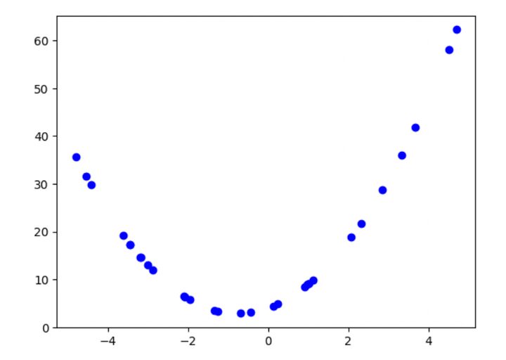
Figure 1: Plot of the second-order polynomial

Here’s the Python code for plotting the equation:

import numpy as np
import matplotlib.pyplot as plt

# Simulating a second-order polynomial with random input values
np.random.seed(42) # For reproducibility
X = np.random.uniform(-5, 5, 30)
y = 2 * X**2 + 3 * X + 4
X = X.reshape(-1, 1)

# Plotting the data
plt.scatter(X,y, color='blue')

Plotting_equation.py hosted with ❤ by GitHub

I have assigned random values to X, which range from -5 to 5 and belong to a uniform distribution. Suppose we are given only this scatter plot (not the equation). With some basic math knowledge, we could identify it as a second-order polynomial. We can even do this visually.

But in real settings, things aren’t that straightforward. Any data we gather or analyze will not form such a clear pattern, and there will be a random component. We term this random component as noise. To know more about noise, you can go through this blog article and also this one.

Adding a Noise Component

When we add a noise component to the above equation, this is how it looks like:

y = 2X² + 3X + 4 + noise

What would its plot look like? Here you go:

Figure 2: Plot of the second-order polynomial with noise

Do you think it’s as easily interpretable as the previous one? Maybe, since we only have 30 data points, the curve still looks somewhat second-orderish! But we’ll need a deeper analysis when we have many data points, and the underlying equation also starts getting more complex.

Here’s the code for generating the above data points and the plot from Figure 2:

# Simulating a second-order polynomial with random input values and noise component
np.random.seed(42) # For reproducibility
X = np.random.uniform(-5, 5, 30)
y = 2 * X**2 + 3 * X + 4 + np.random.normal(0, 10, X.shape[0])
X = X.reshape(-1, 1)

# Plotting the data
plt.scatter(X,y, color='blue')

Second_order_polynomial.py hosted with ❤ by GitHub

Looking closely, you’ll realize that the noise component above belongs to a normal distribution, with mean = 0 and standard deviation = 10.

Splitting into Testing and Training Sets

Let’s now discuss the meaty part. We shall split the above data into train and test sets, with sizes of 20 and 10, respectively. If you aren’t conversant with these basic machine-learning concepts, I recommend skimming through this free book: ML for Trading.

This is what the data looks like after splitting:

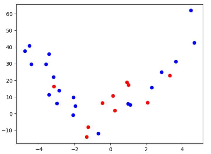
Figure 3: Plot of the second-order polynomial after splitting into train and test data

Here’s the code for the split and the above plot:

from sklearn.model_selection import train_test_split

# Splitting into training and testing sets
X_train, X_test, y_train, y_test = train_test_split(X, y, test_size=10, random_state=42)

# Plotting the data
plt.scatter(X_train, y_train, color='blue')
plt.scatter(X_test, y_test, color='red')

Split_train_test.py hosted with ❤ by GitHub

Fitting Four Different Models to the Data for Illustrating Bias and Variance

After splitting the data, we’ll train four different models with polynomials of order 1, 2, 3, and 10, respectively, and check their accuracies. We’ll do this by using linear regression. We’ll import the “PolynomialFeatures” and “LinearRegression” functionalities from different sub-modules of the scikit-learn library. Let’s see what the four models look like after we fit them on the data, with their respective accuracies:

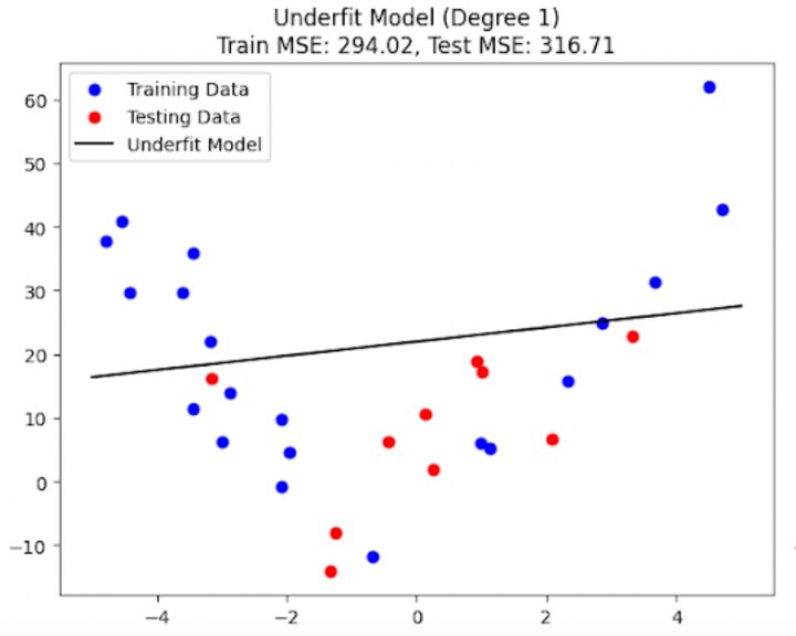
Figure 4a: Underfit model with high bias

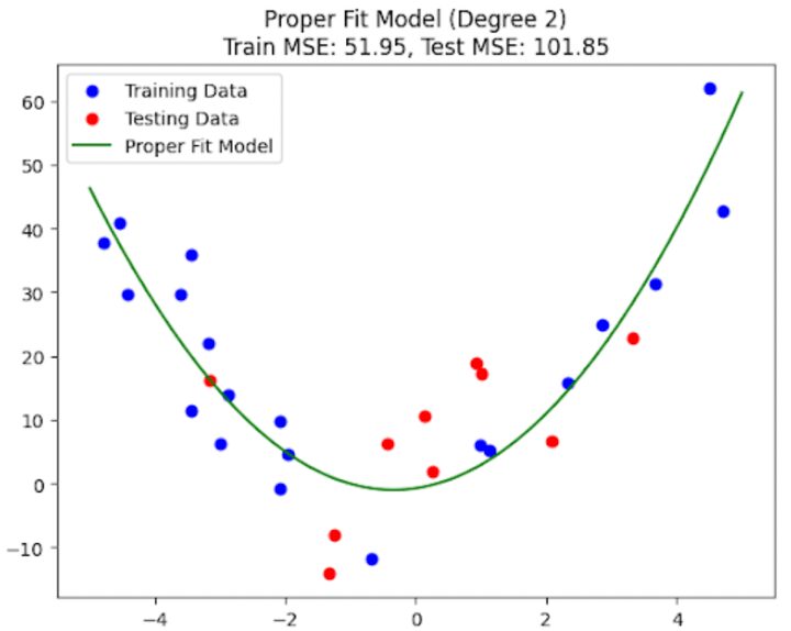
Figure 4b: Properly fit model with low bias and low variance (second order)

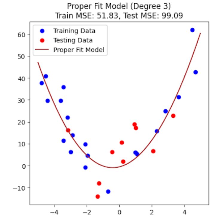
Figure 4c: Properly fit model with low bias and low variance (third order)

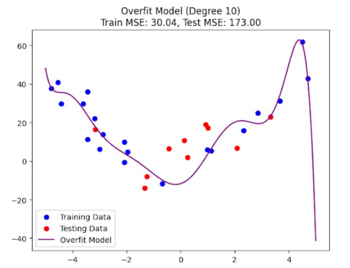
Figure 4d: Overfit model with high variance

The above four plots (Figure 4a to Figure 4d) should give you a clear picture of what it looks like when a machine learning model underfits, properly fits, and overfits on the training data. You might wonder why I’m showing you two plots (and thus two different models) for a proper fit. Don’t worry; I’ll discuss this in a couple of minutes.

For now, here’s the code for training the four models and for plotting them:

from sklearn.preprocessing import PolynomialFeatures
from sklearn.linear_model import LinearRegression
from sklearn.metrics import mean_squared_error

# Generating smooth data for plotting
X_plot = np.linspace(-5, 5, 1000).reshape(-1, 1)

# Function to train and evaluate models
def train_model(degree, X_train, y_train, X_test, y_test):
    poly = PolynomialFeatures(degree)
    X_train_poly = poly.fit_transform(X_train)
    X_test_poly = poly.transform(X_test)
    model = LinearRegression().fit(X_train_poly, y_train)

    # Training and testing errors
    y_train_pred = model.predict(X_train_poly)
    train_error = mean_squared_error(y_train, y_train_pred)
    y_test_pred = model.predict(X_test_poly)
    test_error = mean_squared_error(y_test, y_test_pred)

    # Predicting smooth curve for plotting
    X_plot_poly = poly.transform(X_plot)
    y_plot = model.predict(X_plot_poly)

    return train_error, test_error, y_plot

# Training models
degrees = [1, 2, 3, 10]
results = {}
for degree in degrees:
    train_error, test_error, y_plot = train_model(degree, X_train, y_train, X_test, y_test)
    results[degree] = (train_error, test_error, y_plot)

# Plotting results
plt.figure(figsize=(18, 5))

# Underfit (degree 1)
plt.subplot(1, 4, 1)
plt.scatter(X_train, y_train, color='blue', label='Training Data')
plt.scatter(X_test, y_test, color='red', label='Testing Data')
plt.plot(X_plot, results[1][2], color='black', label='Underfit Model')
plt.title(f'Underfit Model (Degree 1)\nTrain MSE: {results[1][0]:.2f}, Test MSE: {results[1][1]:.2f}')
plt.legend()

# Proper Fit (degree 2)
plt.subplot(1, 4, 2)
plt.scatter(X_train, y_train, color='blue', label='Training Data')
plt.scatter(X_test, y_test, color='red', label='Testing Data')
plt.plot(X_plot, results[2][2], color='green', label='Proper Fit Model')
plt.title(f'Proper Fit Model (Degree 2)\nTrain MSE: {results[2][0]:.2f}, Test MSE: {results[2][1]:.2f}')
plt.legend()

# Proper Fit (degree 3)
plt.subplot(1, 4, 3)
plt.scatter(X_train, y_train, color='blue', label='Training Data')
plt.scatter(X_test, y_test, color='red', label='Testing Data')
plt.plot(X_plot, results[3][2], color='brown', label='Proper Fit Model')
plt.title(f'Proper Fit Model (Degree 3)\nTrain MSE: {results[3][0]:.2f}, Test MSE: {results[3][1]:.2f}')
plt.legend()

# Overfit (degree 10)
plt.subplot(1, 4, 4)
plt.scatter(X_train, y_train, color='blue', label='Training Data')
plt.scatter(X_test, y_test, color='red', label='Testing Data')
plt.plot(X_plot, results[10][2], color='purple', label='Overfit Model')
plt.title(f'Overfit Model (Degree 10)\nTrain MSE: {results[10][0]:.2f}, Test MSE: {results[10][1]:.2f}')
plt.legend()

plt.tight_layout()
plt.show()

Training_the_four_models.py hosted with ❤ by GitHub

Formal Discussion on Bias and Variance

Let’s understand underfitting and overfitting better now.

Underfitting is also termed as “bias”. An underfit model doesn’t align with many points in the training data and carries on its own path. It doesn’t allow the data points to modify itself much. You can think of an underfit model as a person with a mind that’s mostly, if not wholly, closed to the ideas, methods, and opinions of others and always carries a mental bias toward things. An underfit model, or a model with high bias, is simplistic and can’t capture much essence or inherent information in the training data. Thus, it can not generalize well to the testing (unseen) data. Both the training and testing accuracies of such a model are low.

Overfitting is referred to as “variance”. In this case, the model aligns itself with most, if not all, data points in the training set. You can think of a model which overfits as a fickle-minded person who always sways on the opinions and decisions of others, and does not have any conviction of hertheir own. An overfit model, or a model with a high variance, tries to capture every minute detail of the training data, including the noise, so much so that it can’t generalize to the testing (unseen) data. In the case of a model with an overfit, the training accuracy is high, but the testing accuracy is low.

In the case of a properly fit model, we get low errors on both the training and testing data. For the given example, since we already know the equation to be a second-order polynomial, we should expect a second-order polynomial to yield the minimum testing and training errors. However, as you can see from the above results, the third-order polynomial model gives fewer errors on the training and the testing data. What’s the reason for this? Remember the noise term? Yup, that’s the primary reason for this discrepancy. What’s the secondary reason, then? The low number of data points!

Change in Training and Testing Accuracy with Model Complexity

Let’s plot the training and testing accuracies of all four models:

Figure 5: Training and testing errors for all the four models

From Figure 5 above, we can infer the following:

1. The training and testing errors are pretty high for the underfit model.
2. The training and testing errors are around the lowest for the proper fit model/s.
3. The training error is low (even lower than the proper fit models), but the testing error is high.
4. The testing error is higher than the training error in all cases.

Oh, and yes, here’s the code for the above calculation and the plots:

# Calculating training and testing errors for all models
train_errors = [results[degree][0] for degree in degrees]
test_errors = [results[degree][1] for degree in degrees]

# Plotting the training and testing errors
plt.figure(figsize=(8, 6))
plt.plot(degrees, train_errors, marker='o', label='Training Error')
plt.plot(degrees, test_errors, marker='o', label='Testing Error')
plt.xlabel('Model Complexity (Polynomial Degree)')
plt.ylabel('Mean Squared Error')
plt.title('Training and Testing Errors for Different Model Complexities')
plt.xticks(degrees)  # Ensure all degrees are shown on x-axis
plt.legend()
plt.grid(True)
plt.show()

Calculating_training_testing_errors.py hosted with ❤ by GitHub

Mathematical Treatment of Different Error Terms and Decomposition

Now, with that out of the way, let’s proceed towards more mathematical definitions of bias and variance.

Let’s begin with the loss function. In machine learning parlance, the loss function is the function that we desire to minimize. Only after we get the least possible value of the loss function can we say that we have trained or fit the model well.

The mean square error (MSE) is one such loss function. If you’re familiar with the MSE, you’ll know that the lower the MSE, the more accurate the model.

The equation for the MSE is:

Thus,

MSE = Bias² + Variance

From the above equation, it is apparent that to reduce the error, we need to reduce either or both from bias and variance. However, since lowering either of these leads to a rise in the other, we need to develop a combination of both, which yields the minimum value for the MSE. So, if we do that and are lucky, can we end up with an MSE value of 0? Well, not quite! Apart from the bias and variance terms, there’s another term that we need to add here. Owing to the inherent nature of any observed/recorded data, there is some noise in it, which comprises that part of the error we can’t reduce. We term this part as the irreducible error. Thus, the equation for MSE becomes:

MSE = Bias² + Variance + Irreducible Error

Let’s develop an intuition using the same simulated dataset as before.

We shall tweak the equation for MSE:

How and why did we do this? To get into the details, refer to Neural Networks and the Bias/Variance Dilemma” by Stuart German.

Basis the above paper, the equation for the MSE is:

where,

Thus, the bias for each data point is the difference between the mean of all predicted values and the mean of all observed values. Quite intuitively, the lesser this difference, the lesser the bias, and the more accurate the model. But is it really so? Let’s not forget that we increase the variance when we obtain a fit with a low bias.. How do we define the variance in mathematical terms? Here’s the equation:

The MSE comprises the above-defined bias and variance terms. However, since the MSE and variance terms are essentially squares of the differences between different y values, we must do the same to the bias term to ensure dimensional homogeneity.

Thus,

MSE = Bias² + Variance

From the above equation, it is apparent that to reduce the error, we need to reduce either or both from bias and variance. However, since lowering either of these leads to a rise in the other, we need to develop a combination of both, which yields the minimum value for the MSE. So, if we do that and are lucky, can we end up with an MSE value of 0? Well, not quite! Apart from the bias and variance terms, there’s another term that we need to add here. Owing to the inherent nature of any observed/recorded data, there is some noise in it, which comprises that part of the error we can’t reduce. We term this part as the irreducible error. Thus, the equation for MSE becomes:

MSE = Bias² + Variance + IrreducibleError

Let’s develop an intuition using the same simulated dataset as before.

We shall tweak the equation for MSE:

How and why did we do this? To get into the details, refer to Neural Networks and the Bias/Variance Dilemma” by Stuart German.

Basis the above paper, the equation for the MSE is:

where,

We won’t discuss anything more here since it is outside the scope of this blog article. You can refer to the paper cited above for a deeper understanding.

Values of the MSE, Bias, Variance, and Irreducible Error for the Simulated Data, and Their Intuition

We’ll also calculate the bias term and the variance term along with the MSE (using the tweaked formula mentioned above).. This is what the values look like for the testing data:

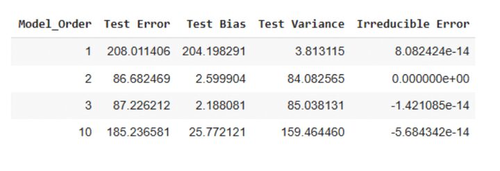
Table 1: Testing errors for simulated data

We can make the following observations from Table 1 above:

1. The test errors are minimal for models with orders 2 and 3.
2. The model with order 0 has the maximum bias term.
3. The model with order 10 has the maximum variance term.
4. The irreducible error is either 0 or negligible.

Here are the corresponding values for the training dataset:

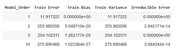
Table 2: Training errors for simulated data

We can make the following observations from Table 2 above:

1. The training errors are higher for the three higher order models than the testing errors.
2. The bias term is negligible for all four models.
3. The error increases with increasing model complexity.

The above three discrepancies can be attributed to our data comprising only 20 train and 10 test data points. How, despite this data sampling, did we not get discrepancies in the test data error calculations? Well, for one, the test data remains unseen by the model, and the model tried to predict values based on what it learned during the training. Secondly, there is an inherent randomness when we work with such small samples, and we may have landed on the luckier side of things with the testing data. Thirdly, we did get a discrepancy, with the irreducible errors being almost 0 in the testing sample. Like I mentioned above, there is always an irreducible error owing to the inherent nature of any data. However, we got no such error since we used data that was simulated by using equations and did not use actual observed data.

The point of the above discussion is not to inspect the values that we got but to derive an intuition of the bias and variance terms. Hope you have a clear picture of these terms now. There’s another term called ‘decomposition’. It simply refers to the fact that we can ‘decompose’ the total error of any model into its error owing to bias, error owing to variance, and the inherent irreducible error.

Here’s the code for getting the above tables:

# Function to train and evaluate models, and demonstrate the bias-variance decomposition
def train_model_decomposition(degree, X_train, y_train, X_test, y_test):
    poly = PolynomialFeatures(degree)
    X_train_poly = poly.fit_transform(X_train)
    X_test_poly = poly.transform(X_test)
    model = LinearRegression().fit(X_train_poly, y_train)

    # Training and testing errors
    y_train_pred = model.predict(X_train_poly)
    train_error = np.mean((y_train_pred - np.mean(y_train))**2)
    train_bias = (np.mean(y_train_pred) - np.mean(y_train))**2
    train_variance = np.mean((y_train_pred - np.mean(y_train_pred))**2)
    y_test_pred = model.predict(X_test_poly)
    test_error = np.mean((y_test_pred - np.mean(y_test))**2)
    test_bias = (np.mean(y_test_pred) - np.mean(y_test))**2
    test_variance = np.mean((y_test_pred - np.mean(y_test_pred))**2)

    # Predicting smooth curve for plotting
    X_plot_poly = poly.transform(X_plot)
    y_plot = model.predict(X_plot_poly)

    return train_error, train_bias, train_variance, test_error, test_bias, test_variance, y_plot

# Training models
degrees_decomposition = [1, 2, 3, 10]
results_decomposition = {}
for degree in degrees_decomposition:
    train_error, train_bias, train_variance, test_error, test_bias, test_variance, y_plot = train_model_decomposition(degree, X_train, y_train, X_test, y_test)
    results_decomposition[degree] = (train_error, train_bias, train_variance, test_error, test_bias, test_variance, y_plot)

Training_models_BVT.py hosted with ❤ by GitHub

import pandas as pd

# Creating a dataframe for the testing error decomposition
df_test = pd.DataFrame({
    "Model_Order": [1, 2, 3, 10],
    "Test Error": [results_decomposition[1][3], results_decomposition[2][3], results_decomposition[3][3], results_decomposition[10][3]],
    "Test Bias": [results_decomposition[1][4], results_decomposition[2][4], results_decomposition[3][4], results_decomposition[10][4]],
    "Test Variance": [results_decomposition[1][5], results_decomposition[2][5], results_decomposition[3][5], results_decomposition[10][5]]
})

# Calculating the irreducible testing error
df_test['Irreducible Error'] = df_test['Test Error'] - df_test['Test Bias'] - df_test['Test Variance']
df_test

# Creating a dataframe for the training error decomposition
df_train = pd.DataFrame({
    "Model_Order": [1, 2, 3, 10],
    "Train Error": [results_decomposition[1][0], results_decomposition[2][0], results_decomposition[3][0], results_decomposition[10][0]],
    "Train Bias": [results_decomposition[1][1], results_decomposition[2][1], results_decomposition[3][1], results_decomposition[10][1]],
    "Train Variance": [results_decomposition[1][2], results_decomposition[2][2], results_decomposition[3][2], results_decomposition[10][2]]
})

# Calculating the irreducible training error
df_train['Irreducible Error'] = df_train['Train Error'] - df_train['Train Bias'] - df_train['Train Variance']
df_train

Error_calculation.py hosted with ❤ by GitHub

Till Next Time

Phew! That was a lot! We should stop here for now. In the second part, we’ll explore how to predict market prices and build trading strategies by employing bias-variance decomposition.

Visit QuantInsti to download the Bias Variance Decomposition – Python notebook and for additional insights on this topic.