
- Solve real problems with our hands-on interface
- Progress from basic puts and calls to advanced strategies
Interactive Options Course

Posted August 6, 2025 at 4:42 pm
The article “Bayesian Statistics in Finance: A Trader’s Guide to Smarter Decisions” was originally published on QuantInsti blog.
Bayesian statistics offers a flexible, adaptive framework for making trading decisions by updating beliefs with new market data. Unlike traditional models, Bayesian methods treat parameters as probabilities, making them ideal for uncertain, fast-changing financial markets.
They’re used in risk management, model tuning, classification, and incorporating expert views or alternative data. Tools like PyMC and Bayesian optimisation make it accessible for quants and traders aiming to build smarter, data-driven strategies.
This blog covers:
Want to ditch rigid trading models and truly harness the power of incoming market information? Imagine a system that learns and adapts, just like you do, but with the precision of mathematics. Welcome to the world of Bayesian statistics, a game-changing framework for algorithmic traders. It’s all about making informed decisions by logically blending what you already know with what the market is telling you right now.
Let’s explore how this can sharpen your trading edge!
This approach contrasts with the traditional, or “frequentist,” view of probability, which often sees probabilities as long-run frequencies of events and parameters as fixed, unknown constants (Neyman, 1937).
Bayesian statistics, on the other hand, treats parameters themselves as random variables about which we can have beliefs and update them as more data comes in (Gelman et al., 2013). Honestly, this feels tailor-made for trading, doesn’t it? After all, market conditions and relationships are hardly ever set in stone. So, let’s jump in and see how you can use Bayesian stats to get a leg up in the fast-paced world of finance and algorithmic trading.
To fully grasp the Bayesian methods discussed in this blog, it is important to first establish a foundational understanding of probability, statistics, and algorithmic trading.
For a conceptual introduction to Bayesian statistics, Bayesian Inference Methods and Equation Explained with Examples offers an accessible explanation of Bayes’ Theorem and how it applies to uncertainty and decision-making, foundational to applying Bayesian models in markets.
Prior Beliefs, New Evidence, Updated Beliefs
Okay, let’s break down the fundamental magic of Bayesian statistics. At its core, it’s built on a wonderfully simple yet incredibly powerful idea: our understanding of the world is not static; it evolves as we gather more information.
Think about it like this: you’ve got a new trading strategy you’re mulling over.
This whole process of tweaking your beliefs based on new info is neatly wrapped up and formalised by what is called the Bayes’ Theorem.
Bayes’ Theorem: The Engine of Bayesian Learning
So, Bayes’ Theorem is the actual formula that ties all these pieces together. If you have a hypothesis (let’s call it H) and some evidence (E), the theorem looks like this:
Bayes’ Theorem:

Where:
Let’s try to make this less abstract with a quick trading scenario.
Example: Is a News Event Bullish for a Stock?
Suppose a company is about to release an earnings report.
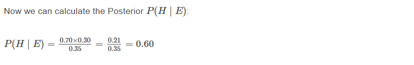
Boom! After seeing that 1% price jump, your belief that the earnings report will be a positive surprise has shot up from 30% to 60%! This updated probability can then inform your trading decision, perhaps you’re now more inclined to buy the stock or adjust an existing position.
Of course, this is a super-simplified illustration. Real financial models are juggling a significantly greater number of variables and much more complex probability distributions. But the beautiful thing is, that core logic of updating your beliefs as new info comes in? That stays exactly the same.

Financial markets are a wild ride, full of uncertainty, constantly changing relationships (non-stationarity, if you want to get technical), and often, not a lot of data for those really rare, out-of-the-blue events. Bayesian methods offer several advantages in this environment:
Alright, enough theory! Let’s get down to brass tacks. How can you actually use Bayesian statistics in your trading algorithms?
So many trading models lean heavily on parameters – like the lookback window for your moving average, the speed of mean reversion in a pairs trading setup, or the volatility guess in an options pricing model. But here’s the catch: market conditions are always shifting, so parameters that were golden yesterday might be suboptimal today.
This is where Bayesian methods are super handy. They let you treat these parameters not as fixed numbers, but as distributions that get updated as new data rolls in. Imagine you’re estimating the average daily return of a stock.
Hot Trend Alert: Techniques like Kalman Filters (which are inherently Bayesian) are widely used for dynamically estimating unobserved variables, like the “true” underlying price or volatility, in noisy market data (Welch & Bishop, 2006). Another area is Bayesian regression, where the regression coefficients (e.g., the beta of a stock) are not fixed points but distributions that can evolve.
For more on regression in trading, you might want to check out how Regression is Used in Trading.
Simplified Python Example: Updating Your Belief about a Coin’s Fairness (Think Market Ups and Downs)
Let’s say we want to get a handle on the probability of a stock price going up (we’ll call it ‘Heads’) on any given day. This is a bit like trying to figure out if a coin is fair or biased.
Python Code:
# Import necessary library for statistical distributions
import scipy.stats as stats
# Import numpy for numerical operations
import numpy as np


# --- Prior Beliefs ---
# We'll use a Beta distribution to represent our belief about the probability of an 'up' day (p_up).
# The Beta distribution is defined by two parameters: alpha (successes) and beta (failures).
# Let's start with a relatively uninformative prior: alpha_prior = 1, beta_prior = 1
# This prior is equivalent to assuming we've seen one 'up' day and one 'down' day.
alpha_prior = 1
beta_prior = 1
print(f"Initial Prior: Alpha={alpha_prior}, Beta={beta_prior}")


# --- Observed Data (New Evidence) ---
# Suppose we observe the market for 10 days and see:
# 6 'up' days (1) and 4 'down' days (0)
# This is our new evidence from the market.
market_data = [1, 1, 0, 1, 0, 1, 1, 0, 1, 0] # 1 for up, 0 for down/flat
num_up_days = sum(market_data)
num_down_days = len(market_data) - num_up_days
print(f"Observed Data: {num_up_days} 'up' days, {num_down_days} 'down' days")


# --- Update Beliefs (Calculate Posterior) ---
# For a Beta prior and Binomial likelihood (like coin flips), the posterior is also a Beta distribution.
# The posterior alpha is prior alpha + number of new successes (up days).
alpha_posterior = alpha_prior + num_up_days
# The posterior beta is prior beta + number of new failures (down days).
beta_posterior = beta_prior + num_down_days
print(f"Posterior Belief: Alpha={alpha_posterior}, Beta={beta_posterior}")


# --- Interpretation of Posterior ---
# The mean of this Beta distribution is our updated estimate for p_up.
# Mean of Beta(alpha, beta) = alpha / (alpha + beta)
estimated_p_up = alpha_posterior / (alpha_posterior + beta_posterior)
print(f"Updated Estimated Probability of an 'Up' Day: {estimated_p_up:.2f}")


# We can also get the credible interval (Bayesian equivalent of confidence interval)
# For example, a 95% credible interval
# This tells us the range within which we are 95% confident the true p_up lies.
credible_interval = stats.beta.interval(0.95, alpha_posterior, beta_posterior)
print(f"95% Credible Interval for p_up: ({credible_interval[0]:.2f}, {credible_interval[1]:.2f})")


#Visualizing the results
import matplotlib.pyplot as plt


# Define a range of possible p_up values from 0 to 1
p_values = np.linspace(0, 1, 100)


# Compute the Beta PDF (probability density function) for the prior
prior_pdf = stats.beta.pdf(p_values, alpha_prior, beta_prior)


# Compute the Beta PDF for the posterior
posterior_pdf = stats.beta.pdf(p_values, alpha_posterior, beta_posterior)


# Plot the prior and posterior distributions
plt.figure(figsize=(10, 6))


# Plot the prior in blue
plt.plot(p_values, prior_pdf, label='Prior Beta(1,1)', linestyle='--', color='blue')


# Plot the posterior in green
plt.plot(p_values, posterior_pdf, label=f'Posterior Beta({alpha_posterior},{beta_posterior})', color='green')


# Add title and labels
plt.title("Prior vs Posterior Belief About Probability of an 'Up' Day", fontsize=14)
plt.xlabel("Probability of 'Up' Day (p_up)")
plt.ylabel("Density")
plt.legend()
plt.grid(True)


# Show the plot
plt.tight_layout()
plt.show()
Prior_vs_posterior.py hosted with ❤ by GitHub
Output:
Initial Prior: Alpha=1, Beta=1
Observed Data: 6 'up' days, 4 'down' days
Posterior Belief: Alpha=7, Beta=5
Updated Estimated Probability of an 'Up' Day: 0.58
95% Credible Interval for p_up: (0.31, 0.83)

In this code:
The graph provides a clear visual for this belief-updating process. The flat blue line represents our initial, uninformative prior, where any probability for an ‘up’ day was considered equally likely. In contrast, the orange curve is the posterior belief, which has been sharpened and informed by the observed market data. The peak of this new curve, centered around 0.58, represents our updated, most probable estimate, while its more concentrated shape signifies our reduced uncertainty now that we have evidence to guide us.
This is a toy example, but it shows the mechanics of how beliefs get updated. In algorithmic trading, this could be applied to the probability of a profitable trade for a given signal or the probability of a market regime persisting.
Next up, let’s talk about Naive Bayes. It’s a straightforward probabilistic classifier that uses Bayes’ theorem, but with a “naive” (or let’s say, optimistic) assumption that all your input features are independent of each other. Despite its simplicity, it can be surprisingly effective for tasks like classifying whether the next day’s market movement will be ‘Up’, ‘Down’, or ‘Sideways’ based on current indicators. (Rish, 2001)
Here’s how it works (conceptually):
Python Snippet Idea (Just a concept, you’d need sklearn for this):
Python Code:
# Import the Gaussian Naive Bayes classifier
from sklearn.naive_bayes import GaussianNB
# Import train_test_split for splitting data
from sklearn.model_selection import train_test_split
# Import accuracy_score to evaluate the model
from sklearn.metrics import accuracy_score
# Import numpy for creating sample data
import numpy as np


# --- Assume X contains your features (e.g., RSI, MACD values) ---
# X would be a 2D array where rows are observations and columns are features.
# Let's create some dummy data for demonstration:
# Say we have 100 samples and 2 features.
X_dummy = np.random.rand(100, 2) # 100 days, 2 features (e.g., RSI, %change)


# --- Assume y contains your target variable (0 for Down, 1 for Up) ---
# y would be a 1D array.
# Let's create dummy target data, roughly balanced.
y_dummy = np.random.randint(0, 2, 100) # 0 for Down/Flat, 1 for Up


# Split data into training and testing sets
# This helps evaluate how well the model generalizes to unseen data.
X_train, X_test, y_train, y_test = train_test_split(X_dummy, y_dummy, test_size=0.3, random_state=42)


# Initialize the Gaussian Naive Bayes classifier
# GaussianNB is used when features are continuous and assumed to follow a Gaussian distribution.
model = GaussianNB()


# Train the model using the training data
# The model learns the probabilities P(Feature|Class) and P(Class) from this data.
model.fit(X_train, y_train)


# Make predictions on the test data
# The model applies Bayes' theorem to predict the class for each sample in X_test.
y_pred = model.predict(X_test)


# --- Evaluate the model ---
# Calculate the accuracy: proportion of correct predictions.
accuracy = accuracy_score(y_test, y_pred)
print(f"Naive Bayes Classifier Accuracy (on dummy data): {accuracy:.2f}")


# --- To predict for new, unseen data ---
# new_market_data would be a 2D array with the latest feature values, e.g., [[current_RSI, current_MACD]]
# new_prediction = model.predict(new_market_data)
# print(f"Prediction for new data: {'Up' if new_prediction[0] == 1 else 'Down'}")
Naives_Bayes_classifier.py hosted with ❤ by GitHub
Output:
Naive Bayes Classifier Accuracy (on dummy data): 0.43
This accuracy score of 0.43 indicates the model correctly predicted the market’s direction 43% of the time on the unseen test data. Since this result is below 50% (the equivalent of random chance), it suggests that, with the current dummy data and features, the model does not demonstrate predictive power. In a real-world application, such a score would signal that the chosen features or the model itself may not be suitable, prompting a re-evaluation of the approach or further feature engineering.
This little snippet gives you the basic flow. Building a real Naive Bayes classifier for trading takes careful thought about which features to use (that’s “feature engineering”) and rigorous testing (validation). That “naive” assumption that all features are independent might not be perfectly true in the messy, interconnected world of markets, but it often gives you a surprisingly good starting point or baseline model.
Curious about where to learn all this? Don’t worry, friend, we’ve got you covered! Check out this course.
You’ve probably heard of Value at Risk (VaR), it’s a common way to estimate potential losses. But traditional VaR calculations can sometimes be a bit static or rely on simplistic assumptions. Bayesian VaR allows for the incorporation of prior beliefs about market volatility and tail risk, and these beliefs can be updated as new market shocks occur. This can lead to risk estimates that are more responsive and robust, especially when markets get choppy.
For instance, if a “black swan” event occurs, a Bayesian VaR model can adapt its parameters much more quickly to reflect this new, higher-risk reality. A purely historical VaR, on the other hand, might take a lot longer to catch up.
Finding those “just right” parameters for your trading strategy (like the perfect entry/exit points or the ideal lookback period) can feel like searching for a needle in a haystack. Bayesian optimisation is a seriously powerful technique that can help here. It cleverly uses a probabilistic model (often a Gaussian Process) to model the objective function (like how profitable your strategy is for different parameters) and selects new parameter sets to test in a way that balances exploration (trying new areas) and exploitation (refining known good areas) (Snoek et al., 2012). This can be much more efficient than just trying every combination (grid search) or picking parameters at random.
Hot Trend Alert:Bayesian optimisation is a rising star in the broader machine learning world and is incredibly well-suited for fine-tuning complex algorithmic trading strategies, especially when running each backtest takes a lot of computational horsepower.
These days, quants are increasingly looking at “alternative data” sources, things like satellite images, the general mood on social media, or credit card transaction trends. Bayesian methods give you a really natural way to integrate such diverse and often unstructured data with traditional financial data. You can set your priors based on how reliable or strong you think the signal from an alternative data source is.
And it’s not just about new data types. What if a seasoned portfolio manager has a strong conviction about a particular sector because of some geopolitical development that’s difficult to quantify? That “expert opinion” can actually be formalised into a prior distribution, allowing it to influence the model’s output right alongside the purely data-driven signals.
While Bayesian methods have been around in finance for a while, a few areas are really heating up and getting a lot of attention lately:
Like any powerful tool, Bayesian methods come with their own set of pros and cons.
Advantages:
Limitations:
Q. What makes Bayesian statistics different from traditional (frequentist) methods in trading?
Bayesian statistics treats model parameters as random variables with a and allows beliefs to be updated with new data. In contrast, frequentist methods assume parameters are fixed and require large data samples. Bayesian thinking is more dynamic and well-suited to the non-stationary, uncertain nature of financial markets.
Q. How does Bayes’ Theorem help in trading decisions? Can you give an example?
Bayes’ Theorem is used to update probabilities based on new market information. For example, if a stock price jumps 1% before earnings, and past data suggests this often precedes a positive surprise, Bayes’ Theorem helps revise your confidence in that hypothesis, turning a 30% belief into 60%, which can directly influence your trade.
Q. What are priors and posteriors in Bayesian models, and why do they matter in finance?
A prior reflects your initial belief (from past data, theory, or expert views), while a posterior is the updated belief after considering new evidence. Priors help improve performance in low-data or high-uncertainty situations and allow integration of alternative data or human intuition in financial modelling.
Q. What types of trading problems are best suited for Bayesian methods?
Bayesian techniques are ideal for:
Q. Can Bayesian methods work with limited or noisy market data?
Yes! Bayesian methods shine in low-data environments by incorporating informative priors. They also handle uncertainty naturally, representing beliefs as distributions rather than fixed values, crucial when modelling rare market events or new assets.
Q. How is Bayesian optimisation used in trading strategy design?
Bayesian optimisation is used to tune strategy parameters (like entry/exit thresholds) efficiently. Instead of brute-force grid search, it balances exploration and exploitation using a probabilistic model (example, Gaussian Processes), making it perfect for costly backtesting environments.
Q. Are simple models like Naive Bayes really useful in trading?
Yes, Naive Bayes classifiers can serve as lightweight baseline models to predict market direction using indicators like RSI, MACD, or sentiment scores. While the assumption of independent features is simplistic, these models can offer fast and surprisingly solid predictions, especially with well-engineered features.
Q. How does Bayesian thinking enhance risk management?
Bayesian models, like Bayesian VaR (a, update risk estimates dynamically as new data (or shocks) arrive, unlike static historical models. This makes them more adaptive to volatile conditions, especially during rare or extreme events.
Q. What tools or libraries are used to build Bayesian trading models?
Popular tools include:
Q. How can I get started with Bayesian methods in trading?
Start with small projects:
So, there you have it! Bayesian statistics offers an incredibly powerful and flexible way to navigate the unavoidable uncertainties that come with financial markets. By giving you a formal way to blend your prior knowledge with new evidence as it streams in, it helps traders and quants build algorithmic strategies that are more adaptive, robust, and insightful.
While it’s not a magic bullet, understanding and applying Bayesian principles can help you move beyond rigid assumptions and make more nuanced, probability-weighted decisions. Whether you’re tweaking parameters, classifying market conditions, keeping an eye on risk, or optimising your overall strategy, the Bayesian approach encourages a mindset of continuous learning, and that’s absolutely vital for long-term success in the constantly shifting landscape of algorithmic trading.
Start small, perhaps by experimenting with how priors impact a simple estimation, or by trying out a Naive Bayes classifier. As you grow more comfortable, the rich world of Bayesian modeling will open up new avenues for enhancing your trading edge.
If you’re serious about taking your quantitative trading skills to the next level, consider Quantra’s specialised courses like “Machine Learning & Deep Learning for Trading” to enhance Bayesian techniques, or EPAT for comprehensive, industry-leading algorithmic trading certification. These equip you to tackle complex markets with a significant edge.
Keep learning, keep experimenting!
For a structured and applied learning path with Quantra, start with Python for Trading: Basic, then move to Technical Indicators Strategies in Python.
For machine learning, explore the Machine Learning & Deep Learning in Trading: Beginners learning track, which provides practical hands-on insights into implementing models like Bayesian classifiers in financial markets.
If you’re a serious learner, you can take the Executive Programme in Algorithmic Trading (EPAT), which covers statistical modelling, machine learning, and advanced trading strategies with Python.
Information posted on IBKR Campus that is provided by third-parties does NOT constitute a recommendation that you should contract for the services of that third party. Third-party participants who contribute to IBKR Campus are independent of Interactive Brokers and Interactive Brokers does not make any representations or warranties concerning the services offered, their past or future performance, or the accuracy of the information provided by the third party. Past performance is no guarantee of future results.
This material is from QuantInsti and is being posted with its permission. The views expressed in this material are solely those of the author and/or QuantInsti and Interactive Brokers is not endorsing or recommending any investment or trading discussed in the material. This material is not and should not be construed as an offer to buy or sell any security. It should not be construed as research or investment advice or a recommendation to buy, sell or hold any security or commodity. This material does not and is not intended to take into account the particular financial conditions, investment objectives or requirements of individual customers. Before acting on this material, you should consider whether it is suitable for your particular circumstances and, as necessary, seek professional advice.
Options involve risk and are not suitable for all investors. For information on the uses and risks of options, you can obtain a copy of the Options Clearing Corporation risk disclosure document titled Characteristics and Risks of Standardized Options by going to the following link ibkr.com/occ. Multiple leg strategies, including spreads, will incur multiple transaction costs.


Join The Conversation
For specific platform feedback and suggestions, please submit it directly to our team using these instructions.
If you have an account-specific question or concern, please reach out to Client Services.
We encourage you to look through our FAQs before posting. Your question may already be covered!