Introduction

The post “Trading Mid-Frequency and RV like a Pro (Part 1): Identifying Mean-Reversion with Statistical Tests” was originally published on the Objectively Random Blog.

Mean reversion is one of the most important time-series features in finance. Most relative value trades require some form of mean-reversion. Most mid-frequency futures trading involves mean-reversion. Most market-making PnL is based on mean-reversion.

We all know what it is. And in fact, it is usually possible to identify mean-reverting series. The eyeball test just works. If it crosses zero enough times, it probably mean-reverts. It can’t wander. It can’t drift off. It should find its way back down again whenever it’s up, or find its way back up again whenever it’s down.

Eyeballs don’t scale, though, so it is always handy to have a statistical test.

For mean-reversion there are a few in common use:

The Augmented Dickey-Fuller Test (ADF Test)

The idea is if it mean reverts, the AR(1) coefficient will be negative, i.e.,

$$\mathrm{\Delta }{y}_t=\beta y_{t-1}+{\gamma }_1\mathrm{\Delta }{y}_{t-1}+{\gamma }_2\mathrm{\Delta }{y}_{t-2}+\dots \mathrm{\Delta }{y}_{t-k}+{ϵ}_t$$

The extra terms with $\gamma$ are meant to model more complex time-series phenomena. The most important term is $\beta$ and we want to ensure $\beta <0$ (mean-reverting) vs $\beta =0$ (non-stationary). Typically we would choose to use a t-test for testing whether a coefficient is non-zero. But the typical t-distribution is meant to be the distribution of the t-test under the null-hypothesis. That works for regular regressions. But for time-series under the null hypothesis, the t-test does not have a T-distribution. Rather it has what is known as a Dickey-Fuller Distribution. This is only characterised in the large-sample limit (i.e, as the time series sample size $T\to \mathrm{\infty }$ or by simulation). In large-sample the distribution is characterised by

$$t_{\rho }=\frac{\hat{\beta }}{SE(\hat{\beta })}⟹\frac{{\int }_0^{1}W(t)dW(t)}{(\int W^2(t)dt{)}^{3/2}}$$

This distribution is known as the Dickey-Fuller distribution, and it is a non-standard (and left-tailed) distribution, typically tabulated in statistical packages.

The resulting test is known as the Augmented Dickey Fuller Test. It is known as a unit-root test because the null-hypothesis $H_0:\beta =0$ corresponds to a unit-root in the ARMA process, i.e.,

$$y_t=a_1{y}_{t-1}+a_2{y}_{t-2}+\cdots +a_k{y}_{t-k}+{ϵ}_t,$$

that one the roots of the characteristic polynomial is on the unit circle, similar to a Brownian motion.

In practice, since there are as many tests as there are lag-lengths k, automated ADF tests typically use a lag-length selection criterion, such as the Akaike Information Criterion (AIC) or the Bayesian Information Criterion (BIC), to select the lag-length k. Only after the lag-length is selected, the ADF test is performed.

The ADF test is known to have relatively low power, i.e., it is not very good at detecting mean-reversion when it exists (some truly mean-reverting series will be rejected).

Nyblom-Mäkaläinen Test and KPSS Test

The other standard test for mean-reversion is the Nyblom-Mäkaläinen test, available in most stats packages in its more common and general form, the KPSS test.

The standard version is based on a state-space model,

$$\begin{array}{rc}{y}_t& ={\mu }_t+{ϵ}_t\\ {\mu }_t& ={\mu }_{t-1}+{\delta }_t\end{array}$$

also known as the local level model, where $y_t$ is the time series we are testing for mean-reversion, ${\mu }_t$ is the time-varying mean, ${ϵ}_t$ is the noise in the series, and ${\delta }_t$ is the noise in the mean.

Typically we assume ${ϵ}_t\sim \mathcal{N}(0,{\sigma }_{ϵ}^2)$ and ${\delta }_t\sim \mathcal{N}(0,{\sigma }_{\delta }^2)$ are independent.

We can see that $y$ has a unit root when ${\sigma }_{\delta }^2>0$. Consequently, the null-hypothesis for this mean-reversion test is that

$$H_0:{\sigma }_{\delta }^2>0.$$

The Nyblom-Mäkaläinen test is a test for the null-hypothesis that the series is stationary, i.e., it does not have a unit root. This test was originally proposed by Nyblom and Mäkaläinen in 1983, and it is also known as the KPSS test, after Kwiatkowski, Phillips, Schmidt, and Shin who introduced a non-parametric (and more robust version of) it in 1992.

The test statistic is computed as follows: we estimate the state-space model, and then compute the residuals $\widehat{{ϵ}_t}$ from the model. Then we compute the test statistic as follows. Let $e(t)$ be the residuals from regressing $y_t$ on a constant.

We compute the partial sums $S_t=\sum _{s=1}^{t}e(s)$, then the test statistic is given by $\text{KPSS}=\frac{1}{T^2}\sum _{t=1}^T(\sum _{s=1}^T{\widehat{ϵ}}_s{)}^2/{\sigma }_{ϵ}^2$ where $T$ is the sample size, ${\sigma }_{ϵ}^2$ is the variance of the residuals $\widehat{{ϵ}_t}$ (i.e., the standard single period estimator).

The KPSS test is a stationarity test because the null-hypothesis $H_0:{\sigma }_{\delta }^2=0$ corresponds to the series being stationary, i.e., it does not have a unit root.o The large-sample limit of the KPSS test statistic is known, as well as approximate critical values for the test statistic.

The KPSS test is also known to have low power, i.e., it is not very good at detecting unit-roots when they exist (some truly non-stationary series will be accepted as being mean-reverting). Some practitioners consider using it in conjunction with the ADF test, although the results are mixed (see Maddala and Kim, 1998 for more).

Variance Ratio Tests

The variance ratio test is based on the idea that if a series is mean-reverting, then the variance of multi-period returns, when scaled should be smaller than the variance of a random walk.

For a random walk, the variance of the $k$-period return is given by $$\text{Var}(y_{t+k}-y_t)=k{\sigma }^2$$ where ${\sigma }^2$ is the variance of the series. The resulting test statistic is given by $$\text{VR}=\frac{\text{Var}(y_{t+k}-y_t)}{k{\sigma }^2}$$ where ${\sigma }^2$ is the variance of the series. The null-hypothesis is that the series is a random walk, i.e., it does not mean-revert and under the null, it should be centered at 1. k and the alternative hypothesis is that the series is mean-reverting. Lo and MacKinlay (1988) showed that the variance ratio test is a consistent test for mean-reversion, i.e., it converges to the true value as the sample size increases. They also tabulated critical values for the test statistic, which can be used to determine whether the series is mean-reverting or not.

Although the variance ratio test is not as widely used as the ADF or KPSS tests, it is still a useful tool for testing mean-reversion in time-series data and in some ways more intuitive. For every horizon k, we can compute a variance ratio. If it is close to 1, then the series is likely a random walk. If it is less than 1, then the series is likely mean-reverting , at least at this horizon. If it is higher than one, it may be trending, again over that horizon.

And while Lo and Mackinlay tabulated the critical values, the variance ratio itself, can be related to returns on MR trading strategies – typically the lower the VR, the better then mean-reversion strategy. We see this in practice for instance, in trading illiquid FX crosses. Typically liquid crosses (vs EUR, USD or JPY) have a VR close to 1, while illiquid G10 crosses (e.g., CHF/NOK, GBP/SEK, CAD/AUD) have a VR well below 1, indicating strong(er) mean-reversion.

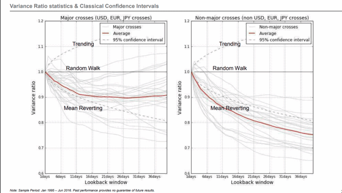
Source: Yahoo Finance

We note that, in the picture, the critical value is more for reference than for specific testing. This is clear when we fix the 30-day horizon (just as an example) and see that the lower the variance ratio, the better the Sharpe ratio of the mean-reversion strategy. The variance ratio is on the x-axis (unlike the previous picture), and we focus entirely on the 30-day horizon.

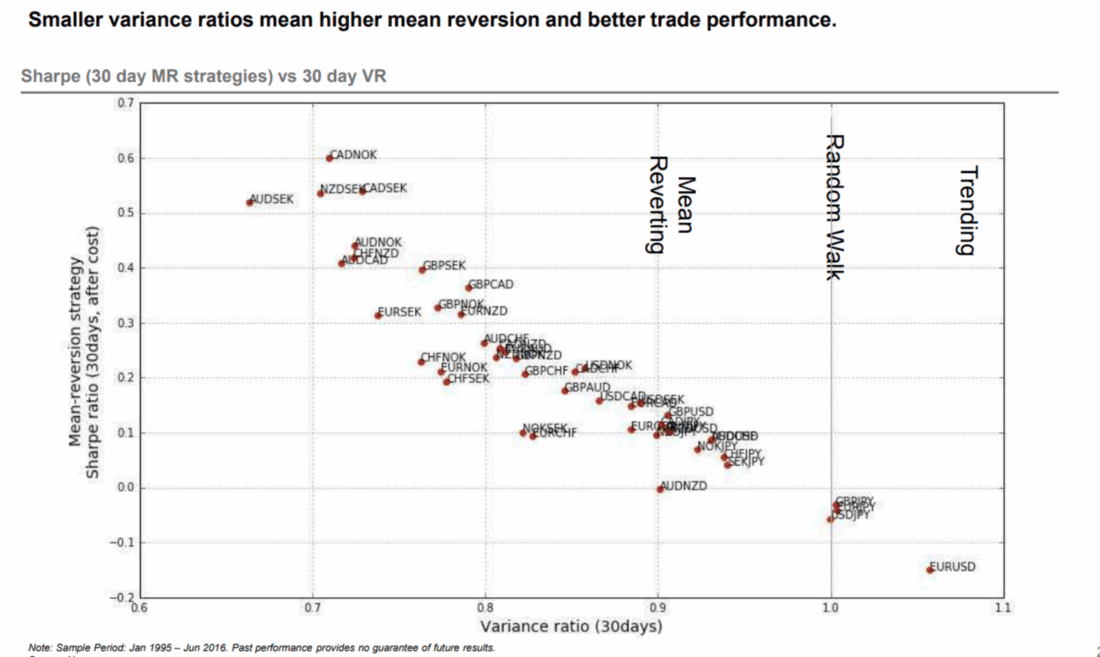
Source: Yahoo Finance

We note that, in the strategy picture, we have not considered trading costs or slippage, which can be significant for mean-reversion strategies.

Mean-Reversion in Practice

Mean-reversion strategies are ubiquitous. However, due to the fact that mean-reversion is a fast phenomenon, transaction costs can be significant.

In terms of a trading strategy, we can think of a mean-reversion strategy as follows.

1. Identify a mean-reverting series, e.g., using the ADF test or KPSS test.
2. Compute the variance ratio for the series, e.g., using the variance ratio test.
3. If the variance ratio is below a certain threshold, then we can consider the series to be mean-reverting, formulating a strategy where we buy when the spread or asset is trading below its mean, and short it when it is trading above its mean.
4. All tests are mere guidance. In reality, a backtest is required to determine the profitability of any strategy, but the tests are a decent starting point for considering whether to spend the time.

Typical strategy weights may involve scaling into a long or a short linear relative to the distance from the mean, or capping and flooring the weights to avoid excessive exposure. Also it is possible to just buy or sell a fixed number of units, when the deviation meets a certain threshold.

Mean-reversion strategies can be applied to levels of a series, to spreads between two series, or to the residuals of a regression between two series. In the latter case, the regression is typically a linear regression, but it can also be a more complex regression, such as a polynomial regression or a spline regression.

Mean-reversion is quite common in pairs trading and relative value trading. Examples include:

1. Futures spreads, between two futures contracts on the same asset (e.g., a slope trade, which tends to mean revert to some typical slope).
2. Pairs trading where two stocks are correlated (e.g., FB and GOOG, or two oil companies, or two banks).
3. Spreads between three assets of fixed weights, e.g., a 1-2-1 butterfly in swaps or US Treasuries, which, over short time-periods tends to mean-revert to a constant ‘fair-value’ spread.
4. A variety of other RV trades such as spread trades (e.g., the swap spread of a given bond relative to its long-term mean), butterflies (as mentioned before), box-trades (e.g., a slope trade in one future vs a slope trade of the same maturities in another future), etc.

Mean-Reversion in a Trading Framework:

In a trading framework, mean-reversion can be thought of as a strategy, effectively a type of model. In the Fundamentals of Algorithmic Trading, we discuss the trading framework in terms of a signal or feature (also known as a factor in the world of Factor-based trading), a model, and a strategy. Each of these forms part of the trading framework, and they are all interlinked.

This chart describes the general flow of a trading framework, from data source to data to feature, etc, where the signal or feature is the input to the model, and the model is the input to the strategy. Sometimes steps are joined together leading to increased efficiency (but increased program complexity!). Sometimes steps are skipped for speed (or done in parallel, e.g., storing the data in a database). The picture does not describe the differences between live-trading and replay or back-testing, but the steps are similar. 

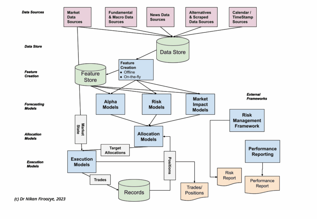
We have not gone into a lot of detail, for instance in execution algorithms, accessing the book, desired position, estimating market impact, choosing order type, placing orders, monitoring them, and allocating fills, etc. The same can be said of each of the steps in the chart, which can be quite complex. We give an overview in the Fundamentals course, and consider in far more detail in the Algorithmic Trading Certificate.

Further Discussion:

While mean-reversion (and the related concept of cointegration, underpinning many pairs-trading and other stats-arb strategies) is a particularly important time-series feature, financial time-series in general have a variety of common aspects which are touched on in the appendix: Financial Time-Series Appendix.

In later posts, we talk about some stylised properties of financial time-series. In particular, the lack of stationarity, or more specifically, the local stationarity, means that mean-reversion must be monitored. In fact, many MR strategies break in time. The levels change, the relationship in spread change, everything changes.

This affects risk management, as well as monitoring the performance of the strategy. In the theoretical world of mean-reversion, stop-losses only hurt performance, but in practice they may be necessary to avoid large losses.

Addressing this is possible using a number of different methods, but most studied include Regime-switching models, and change-point detection methods, as well as (using a slightly different approach), multi-modal models, such as Gaussian Mixture Models, or K-means/K-NN. We will focus on change-point detection, given its similarities to an external statistical risk monitoring system, which can be used to alter estimation techniques and scale strategies. We will discuss this in future blog posts. It is also discussed in the Algorithmic Trading Certificate.

All of this is meant to fit together into forming profitable trading strategies (if it’s not going to be profitable, why do it?). In the course as well we talk more about the properties of certain MR strategies, such as the draw-downs (which are often brutal but brief) etc, and how to scale the strategies as part of a broader portfolio.

References and Further Reading

ADF:

• Dickey, D. A., & Fuller, W. A. (1979). Distribution of the estimators for autoregressive time series with a unit root. Journal of the American Statistical Association, 74(366a), 427-431.
• GS Madalla and I-M Kim (1998), Unit Roots, Cointegration, and Structural Change
• Augmented Dickey-Fuller Test is available in most statistical packages, including Python’s statsmodels and R’s tseries package.

N-M and KPSS:

• Nyblom, J, & Makalainen, E. (1982). Comparisons of Tests for the Presence of Random Walk Coefficients in a Simple Linear Model, Journal of Econometrics, 23(1-2), 145-159. (received 1982, Published online: 2012!)
• Kwiatkowski, D., Phillips, P. C., Schmidt, P., & Shin, Y. (1992). Testing the null hypothesis of stationarity against the alternative of a unit root. Journal of Econometrics, 54(1-3), 159-178.
• KPSS test is available in most statistical packages.

Variance Ratio:

• Lo, A. W., & MacKinlay, A. C. (1988). Stock market prices do not follow random walks: Evidence from a simple specification test. The Review of Financial Studies, 1(1), 41-66. Mingze Gao, VR Tests gives a nice overview.
• VR Tests is available in many statistical packages, including Matlab vratiotest and R vrtest, but only in some github repos for Python.

Recommended Courses:

• Fundamentals of Algorithmic Trading, on the WBS/Quantshub Platform. This introductory course describes the Algo Trading Sector and common roles for quants, before discussing the overall trading framework with a case study on crypto.
• Algorithmic Trading Certificate(ATC): A Practitioner’s Guide For a much more detailed discussion, the Algorithmic Trading Certificate, which is available on the WBS Platform, covers the topic in much more detail, including the statistical tests, the trading strategies, and the implementation details. It is available both as a self-paced course, and a hybrid course with live sessions.

Finally, I am working on a book on Algorithmic Trading, together with Dr Brian Healy, which will cover the topic in much more detail, including the statistical tests, the trading strategies, and the implementation in far more detail.

Objectively Random Blog (Jaynes stan)

• Dr. Nick Firoozye

• firoozye – A blog about quantitative finance, machine learning, and algorithmic trading, with naive forays into philosophy, science and programming.