From Logistic to Random Forests: Mastering Non-linear Regression Models

The post “From Logistic to Random Forests: Mastering Non-linear Regression Models” was originally published on QuantInsti blog.

Ever wish you had a crystal ball for the financial markets? While we can’t quite do that, regression is a super useful tool that helps us find patterns and relationships hidden in data – it’s like being a data detective!

The most common starting point is linear regression, which is basically about drawing the best straight line through data points to see how things are connected. Simple, right?

In Part 1 of this series, we explored ways to make those line-based models even better, tackling things like curvy relationships (Polynomial Regression) and messy data with too many variables (using Ridge and Lasso Regression). We learned how to refine those linear predictions.

But what if a line (even a curvy one) just doesn’t fit? Or what if you need to predict something different, like a “yes” or “no”?

Get ready for Part 2, my friend! Where we venture beyond the linear world and explore a fascinating set of regression techniques designed for different kinds of problems:

1. Logistic Regression: For predicting probabilities and binary outcomes (Yes/No).
2. Quantile Regression: For understanding relationships at different points in the data distribution, not just the average (great for risk analysis!).
3. Decision Tree Regression: An intuitive flowchart approach for complex, non-linear patterns.
4. Random Forest Regression: Harnessing the “wisdom of the crowd” by combining multiple decision trees for accuracy and stability.
5. Support Vector Regression (SVR): A powerful method using “margins” to handle complex relationships, even in high dimensions.

Let’s dive into these powerful tools and see how they can unlock new insights from financial data!

Prerequisites

Hey there! Before we get into the good stuff, it helps to be familiar with a few key concepts. You can still follow along intuitively, but brushing up on these will give you a much better understanding. Here’s what to check out:

1. Statistics and Probability
Know the essentials—mean, variance, correlation, and probability distributions. New to this? Probability Trading is a great intro.

2. Linear Algebra Basics
Basics like matrices and vectors are super useful, especially for techniques like Principal Component Regression.

3. Regression Fundamentals
Get comfy with linear regression and its assumptions. Linear Regression in Finance is a solid starting point.

4. Financial Market Knowledge
Terms like stock returns, volatility, and market sentiment will come up a lot. Statistics for Financial Markets can help you brush up.

5. Explore Part 1 of This Series
Check out Part 1 for an overview of Polynomial, Ridge, Lasso, Elastic Net, and LARS. It’s not mandatory, but it provides excellent context for different regression types.

Once you’re good with these, you’ll be all set to dive deeper into how regression techniques reveal insights in finance. Let’s get started!

What Exactly is Regression Analysis?

At its core, regression analysis models the relationship between a dependent variable (the outcome we want to predict) and one or more independent variables (predictors).

Think of it as figuring out the connection between different things – for instance, how does a company’s revenue (the outcome) relate to how much they spend on advertising (the predictor)? Understanding these links helps you make educated guesses about future outcomes based on what you know.

When that relationship looks like a straight line on a graph, we call it linear regression – nice and simple!

What Makes These Models ‘Non-Linear’?

Good question! In Part 1, we mentioned that ‘linear’ in regression refers to how the model’s coefficients are combined.

Non-linear models, like the ones we’re exploring here, break that rule. Their underlying equations or structures don’t just add up coefficients multiplied by predictors in a simple way. Think about Logistic Regression using that S-shaped curve (sigmoid function) to squash outputs between 0 and 1, or Decision Trees making splits based on conditions rather than a smooth equation, or SVR using ‘kernels’ to handle complex relationships in potentially higher dimensions.

These methods fundamentally work differently from linear models, allowing them to capture patterns and tackle problems (like classification or modelling specific data segments) that linear models often can’t.

Logistic (or Logit) regression

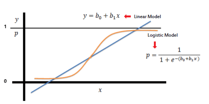
You use Logistic regression when the dependent variable (here, a dichotomous variable) is binary (think of it as a “yes” or “no” outcome, like a stock going up or down). It helps predict the binary outcome of an occurrence based on the given data.

It is a non-linear model that gives a logistic curve with values limited to between 0 and 1. This probability is then compared to a threshold value of 0.5 to classify the data. So, if the probability for a class is more than 0.5, we label it as 1; otherwise, it is 0.

This model is generally used to predict the performance of stocks.

Note: You can not use linear regression here because it could give values outside the 0 to 1 range. Also, the dependent variable can take only two values here, so the residuals won’t be normally distributed about the predicted line.

Want to learn more? Check out this blog for more on logistic regression and how to use Python code to predict stock movement.

Source: https://www.saedsayad.com/logistic_regression.htm

Quantile Regression: Understanding Relationships Beyond the Average

Traditional linear regression models predict the mean of a dependent variable based on independent variables. However, financial time series data often contain skewness and outliers, making linear regression unsuitable.

To solve this problem, Koenker and Bassett (1978) introduced quantile regression. Instead of modeling just the mean, it helps us see the relationship between variables at different points (quantiles and percentiles) in the dependent variable’s distribution, such as:

• 10th percentile (low gains/losses)
• 50th percentile (median returns)
• 99th percentile (high gains/losses)

It estimates different quantiles (like medians or quartiles) of the dependent variables for the given independent variables, instead of just the mean. We call these conditional quantiles.

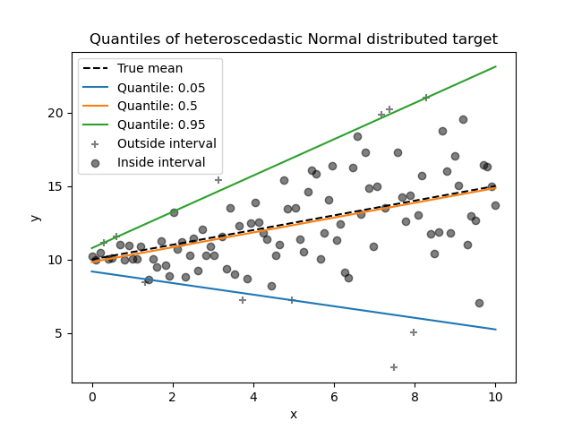
Source: https://scikit-learn.org/stable/auto_examples/linear_model/plot_quantile_regression.html

Like OLS regression coefficients, which show the changes from one-unit changes of the predictor variables, quantile regression coefficients show the changes in the specified quantile from one-unit changes in the predictor variables.

Advantages:

• Robustness to Outliers: According to Lim et al. (2020), regular linear regression assumes errors in the data are normally distributed, but this isn’t reliable when you have outliers or extreme values (“fat tails”).  Quantile regression handles outliers better because it focuses on minimizing absolute errors, not the squared ones like regular regression. This way the influence of extreme values is reduced, providing more reliable estimates in datasets that aren’t really “well behaved” (with heavy tails or skewed distributions) ​
• Estimating Conditional Median: The conditional median is estimated using the median estimator, which minimizes the sum of absolute errors.
• Handling Heteroskedasticity: OLS assumes constant variance of errors (homoskedasticity), but this is often unrealistic. Quantile regression allows for varying error variances, making it effective when predictor variables influence different parts of the response variable’s distribution (Koenker & Bassett, 1978).

Let’s look at an example to better understand how quantile regression works:

Let’s say you’re trying to understand how the overall “mood” of the market (measured by a sentiment index) affects the daily returns of a particular stock. Traditional regression would tell you the average impact of a change in sentiment on the average stock return.

But what if you’re particularly interested in extreme movements? Quantile regression is used here:

• Looking at the 10th percentile: You could use quantile regression to see how a negative shift in market sentiment affects the worst 10% of potential daily returns (the big losses). It might show that negative sentiment has a much stronger negative impact during these extreme downturns than it does on average.
• Looking at the 90th percentile: Similarly, you could see how positive sentiment affects the best 10% of daily returns (the big gains). It might reveal that positive sentiment has a different (possibly larger or smaller) impact on these significant upward swings compared to the average.
• Looking at the 50th percentile (median): You can also see the impact of sentiment on the typical daily return (the median), which might be different from the effect on the average if the return distribution is skewed.

So, instead of just one average effect, quantile regression gives you a more complete picture of how market sentiment influences different parts of the stock’s return distribution, especially the potentially risky extreme losses. Isn’t that great?

Decision Trees Regression: The Flowchart Approach

Imagine trying to predict a numerical value – like the price of something or a company’s future revenue. A Decision Tree offers an intuitive way to do this, working like a flowchart or a game of ‘yes/no’ questions.

A decision tree is divided into smaller and smaller subsets based on certain conditions related to the predictor variables. Think of it like this:

Decision trees  start with your entire dataset and progressively splits it into smaller and smaller subsets at the nodes, thereby creating a tree-like structure. Each of the nodes where the data is split based on a condition is called an internal/split node, and the final subsets are called the terminal/leaf nodes.

In finance, decision trees may be used for classification problems like predicting whether the prices of a financial instrument will go up or down.

Source: https://blog.quantinsti.com/decision-tree/

Decision Tree Regression is when we use a decision tree to predict continuous values (like the price of a house or temperature) instead of categories (like predicting yes/no or up/down).

Here’s how it works in regression:

• The tree asks a series of questions based on the input features (like “Is square footage > 1500?”).
• Based on the answers, the data point moves down the tree until it reaches a leaf.
• In that leaf, the prediction is the average (or sometimes the median) of the actual values from the training data that also landed there.

So, the tree splits the data into groups, and each group gets a fixed number as the prediction.

Things to Watch Out For:

• Overfitting: Decision trees can get too detailed and match the training data too perfectly, making them perform poorly on new, unseen data.
• Instability: Small changes in the training data can sometimes lead to significantly different tree structures. (Techniques like Random Forests and Gradient Boosting often help with this).

You have a full description of the model in this blog and its use in trading in this blog.

To learn more about decision trees in trading check out this Quantra course.

Let’s see a situation where this might be a useful tool:

Imagine you’re trying to predict a company’s sales revenue for the next quarter. You have data on its past performance and factors like: marketing spend in the current quarter, number of salespeople, the company’s industry sector (e.g., Tech, Retail, Healthcare), etc.

The tree might ask:

“Marketing spend > $500k?” If yes, “Industry = Tech?”. Based on the path taken, you land on a leaf.

The prediction for a new company following that path would be the average revenue of all past companies that fell into that same leaf (e.g., the average revenue for tech companies with high marketing spend).

Random forest regression: Wisdom of the Crowd for Predictions

Remember how individual Decision Trees can sometimes be a bit unstable or might overfit the training data? What if we could harness the power of many decision trees instead of relying on just one?

That’s the idea behind Random Forest Regression!

It’s an “ensemble” method, meaning it combines multiple models (in this case, decision trees) to achieve better performance than any single one could alone. You can think of it using the “wisdom of the crowd” principle: instead of asking one expert, you ask many, slightly different experts and combine their insights. Generally, Random Forests perform significantly better than individual decision trees (Breiman, 2001).

How does the forest get “random”?

The “random” part of Random Forest comes from two key techniques used when building the individual trees:

1. Random Data Subsets (Bootstrapping): Each tree in the forest is trained on a slightly different random sample of the original training data. This sample can be chosen “with replacement” (meaning some data points might be selected multiple times, and some might be left out for that specific tree). This ensures each tree sees a slightly different perspective of the data.
2. Random Feature Subsets: When deciding how to split the data at each step inside a tree, the algorithm can only consider a random selection of the input features, not all of them. This stops one or two powerful features from dominating all the trees and encourages diversity.

Making Predictions (Regression = Averaging)

To predict a value for new data, you run it through every tree in the forest. Each tree gives its own prediction. The Random Forest’s final prediction is simply the average of all those individual tree predictions. This averaging smooths things out and makes the model much more stable.

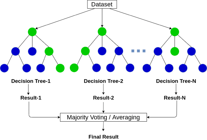
Image representation of a Random forest regressor: Source: https://ai-pool.com/a/s/random-forests-understanding

Why Use Random Forest Regression?

• High Accuracy: Often provides very accurate predictions.
• Robustness: Less prone to overfitting compared to single decision trees and handles outliers reasonably well. (Breiman, L. , 2001)
• Non-linearity: Easily captures complex, non-linear relationships.
• Feature Importance: Can provide estimates of which predictors are most important.

Things to Consider:

• Interpretability: It acts more like a “black box.” It’s harder to understand exactly why it made a specific prediction compared to visualizing a single decision tree.
• Computation: Training many trees can be computationally intensive and require more memory.

Check out this post if you want to learn more about random forests and how they can be used in trading.

Think we’d leave you hanging? No way!

Here’s an example to help you better understand how random forests work in practice:

You want to predict how much a stock’s price will swing (its volatility) next month, using data like recent volatility, trading volume, and market fear (VIX index).

A single decision tree might latch onto a specific pattern in the past data and give a jumpy prediction. A Random Forest approach is more robust:

It builds hundreds of trees. Each tree sees slightly different historical data and considers different feature combinations at each split. Each tree estimates the volatility. The final prediction is the average of all these estimates, giving a more stable and reliable forecast of future volatility than one tree alone could provide.

Support vector regression (SVR): Regression Within a ‘Margin’ of Error

You might be familiar with Support Vector Machines (SVM) for classification. Support Vector Regression (SVR) takes the core ideas of SVM and applies them to regression tasks – that is, predicting continuous numerical values.

SVR approaches regression a bit differently than many other methods. While methods like standard linear regression try to minimize the error between the predicted and actual values for all data points, SVR has a different philosophy.

The Epsilon (ε) Insensitive Tube:

Imagine you’re trying to fit a line (or curve) through your data points. SVR tries to find a “tube” or “street” around this line with a certain width, defined by a parameter called epsilon (ε). The goal is to fit as many data points as possible inside this tube.

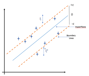
Image representation of Support vector regression: Source: https://www.educba.com/support-vector-regression/

Here’s the key idea: For any data points that fall inside this ε-tube, SVR considers the prediction “good enough” and ignores their error. It only starts penalizing errors for points that fall outside the tube. This makes SVR less sensitive to small errors compared to methods that try to get every point perfect. The regression line (or hyperplane in higher dimensions) runs down the middle of this tube.

Handling Curves (Non-Linearity):

What if the relationship between your predictors and the target variable isn’t straight? SVR uses a “kernel trick”. This is like projecting the data into a higher-dimensional space where a complex, curvy relationship might look like a simpler straight line (or flat plane). By finding the best “tube” in this higher dimension, SVR can effectively model non-linear patterns. Common kernels include linear, polynomial, and RBF (Radial Basis Function). The best choice depends on the data.

Pros:

• Effective in high-dimensional spaces.
• Can model non-linear relationships using kernels.
• The ε-margin offers some robustness to small errors/outliers (Muthukrishnan & Jamila, 2020).

Cons:

• Can be computationally slow on large datasets.
• Performance is sensitive to parameter tuning (choosing ε, a cost parameter C, and the right kernel).
• Interpretability can be less direct than linear regression.

The explanation for the whole model can be found here.

And if you want to learn more about how support vector machines can be used in trading, be sure to check out this blog, my friend!

By now, you probably know how this works, so let’s look at a real-life example that uses SVR:

Think about predicting the price of a stock option (like a call or put). Option prices depend on several complex, non-linear factors: the underlying stock’s price, time left until expiration, expected future volatility (implied volatility), interest rates, etc.

SVR (especially with a non-linear kernel like RBF) is suitable for this. It can capture these complex relationships using the kernel trick. The ε-tube focuses on getting the prediction within an acceptable small range (e.g., predicting the price +/- 5 cents), rather than stressing about tiny deviations for every single option.

Summary

Conclusion

And that concludes our tour through the more diverse landscapes of regression! We’ve seen how Logistic Regression helps us tackle binary predictions, how Quantile Regression gives us insights beyond the average, especially for risk, and how Decision Trees and Random Forests offer intuitive yet powerful ways to model complex, non-linear relationships. Finally, Support Vector Regression provides a unique, margin-based approach practical even in high-dimensional spaces.

From the refined linear models in Part 1 to the varied techniques explored here, you now have a much broader regression toolkit at your disposal. Each model has its strengths and is suited for different financial questions and data challenges.

The key takeaway? Regression is not a one-size-fits-all solution. Understanding the nuances of different techniques allows you to choose the right tool for the job, leading to more insightful analysis and powerful predictive models.

And as you continue learning my friend, don’t just stop at theory. Keep exploring, keep practicing with real data, and keep refining your skills. Happy modeling!

Perhaps you’re keen on a complete, holistic understanding of regression applied directly to trading? In that case, check out this Quantra course.

If you’re serious about taking your skills to the next level, consider QuantInsti’s EPAT program—a solid path to mastering financial algorithmic trading.

With the right training and guidance from industry experts, it can be possible for you to learn it as well as Statistics & Econometrics, Financial Computing & Technology, and Algorithmic & Quantitative Trading. These and various aspects of Algorithmic trading are covered in this algo trading course. EPAT equips you with the required skill sets to build a promising career in algorithmic trading. Be sure to check it out.

References

1. Koenker, R., & Bassett, G. (1978). Regression quantiles. Econometrica, 46(1), 33–50. https://doi.org/10.2307/1913643
2. Lim, D., Park, B., Nott, D., Wang, X., & Choi, T. (2020). Sparse signal shrinkage and outlier detection in high-dimensional quantile regression with variational Bayes. Statistica Sinica, 13(2), 1. https://archive.intlpress.com/site/pub/files/_fulltext/journals/sii/2020/0013/0002/SII-2020-0013-0002-a008.pdf
3. Breiman, L. (2001). Random forests. Machine Learning, 45(1), 5–32. https://link.springer.com/article/10.1023/A:1010933404324
4. Muthukrishnan, R., & Jamila, S. M. (2020). Predictive modeling using support vector regression. International Journal of Scientific & Technology Research, 9(2), 4863–4875. Retrieved from https://www.ijstr.org/final-print/feb2020/Predictive-Modeling-Using-Support-Vector-Regression.pdf