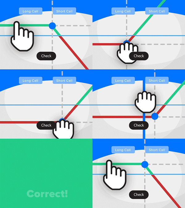
- Solve real problems with our hands-on interface
- Progress from basic puts and calls to advanced strategies
Interactive Options Course

Posted November 16, 2026 at 2:30 pm
This model combines three ideas that are usually met separately. The objective is not a forecast error but a pricing error: the portfolio is treated as a proxy for a stochastic discount factor, and training minimises a regularised Hansen–Jagannathan distance, which has a closed-form first-order condition worth examining before any network is built. The representation is generated rather than predicted: a diffusion model produces a distribution over embeddings instead of a point estimate. And the diffusion prior is retrieved rather than assumed: instead of corrupting towards isotropic noise, the forward process walks towards the mean and spread of the nearest historical episodes, drawn from a context bank under a strict causal mask. The article derives the objective, explains the retrieval-anchored diffusion, gives a complete PyTorch implementation, and uses the worked example to make a point the architecture obscures — that the regularisation term, not the generative machinery, determines how far the output can move from equal weight.
Most machine learning applied to the cross-section of returns is a forecasting exercise: predict next period’s return from characteristics, then build a portfolio from the predictions. The approach has a well-documented problem, which is that predictive R2 in the cross-section of returns is tiny and unstable, and the mapping from a slightly better forecast to a better portfolio is not monotone.
Asset pricing offers a different target. The fundamental condition of no-arbitrage is that there exists a stochastic discount factor M such that every excess return has zero price under it. That condition is a moment restriction, and it can be made into a loss function. A line of work in deep asset pricing (Kozak, Nagel & Santosh, 2020; Chen, Pelger & Zhu, 2024) builds the discount factor as a portfolio and trains a network to minimise the resulting pricing errors. The quantity being optimised is economically meaningful in a way that mean squared forecast error is not.
The second and third ideas address the input side. A single embedding of recent market conditions is a point estimate of something inherently uncertain; a diffusion model (Ho, Jain & Abbeel, 2020) replaces it with a distribution that can be sampled. And since financial history is not long but is repetitive, the prior for that generative model need not be uninformative: if today’s conditions resemble a set of identifiable past episodes, the model can be told to generate near them. Retrieval augmentation of this kind came from language modelling (Lewis et al., 2020) and has been applied to time-series diffusion (Liu et al., 2024). The combination — retrieval-anchored diffusion feeding an SDF objective — is the model described here.
The pricing condition. No-arbitrage requires, for every asset’s excess return yi,
Following the GMM tradition, the discount factor is parameterised as a portfolio of the assets themselves — the discount factor and the efficient portfolio are two views of the same object:
The objective. Squaring and averaging the pricing errors, and adding a ridge penalty on the weights, gives the regularised Hansen–Jagannathan distance that the network minimises:
What that objective actually asks for. This is worth doing by hand before trusting any architecture built on top of it. Differentiating with respect to w and setting the gradient to zero,
The optimum is a ridge-regularised portfolio built from the second-moment matrix and the mean vector — an estimator in the mean–variance family, reached through a pricing argument rather than a utility argument. The derivation treats w as unconstrained; the softmax restricts it to the simplex, which changes the algebra but not the conclusions. Two of those follow immediately and both matter for how the model behaves. The penalty λ governs the size of the tilt: for large λ, w⋆ ≈ λ−1E[y], so the magnitude of the position shrinks like 1/λ — towards zero unconstrained, and towards 1/N on the simplex. And the objective is driven by the first and second moments of returns only; the network’s entire contribution is to make those conditional on the current state.
Weights by construction. The network emits scores and a softmax turns them into weights:
Long-only and fully invested hold exactly. Since an untrained network produces near-uniform scores, training starts at equal weight; combined with the ridge penalty, which on the simplex is minimised at exactly 1/N, the model’s default state is the equal-weighted portfolio and everything it learns is a tilt away from it.
Diffusion, anchored on retrieval. A standard denoising diffusion model corrupts a clean representation x0 towards standard normal noise, with ᾱs the cumulative noise schedule:
Here the terminal distribution is replaced by something informative. Let μR and σR be the mean and standard deviation of the K retrieved neighbours of the current query. The forward process becomes
At s = 0 nothing is corrupted; at the terminal step the sample is drawn from the retrieved distribution rather than from white noise. The reverse chain therefore begins somewhere informative, and the denoiser’s job is the easier one of refining a plausible starting point.
Causal retrieval. The bank stores past segments as key–value pairs, each stamped with the period in which its information set ends. A query at t ranks entries by cosine similarity and takes the top K, but only among entries whose stamp is at or before t:
This mask is not a detail. Retrieval is precisely the mechanism by which a model of this shape can see the future, and the whole construction is only meaningful if the mask is airtight.
Training and assembly. The denoiser is trained to recover the clean embedding while the allocation head is trained on the pricing loss, with one coefficient balancing them: L = LSDF + ρ Ldiff. At inference the reverse chain is run several times and averaged, and the denoised channels are mixed with the raw query through a single interpolation parameter, z = (1 − γ)(q̂ + ĉ) + γ q, where γ controls how much of the generated representation is trusted against the directly encoded one.
PyTorch. The four blocks are the objective, the retrieval bank, the retrieval-anchored diffusion, and the assembled model.
The objective. Six lines. Everything derived in Section 2 is in them, and the ridge coefficient lam is the parameter that decides how far the model may move from equal weight.
import numpy as np
import torch
import torch.nn as nn
import torch.nn.functional as F

def sdf_loss(scores, y, lam=1e-2):
    """Regularised Hansen-Jagannathan distance of a long-only, fully invested book.

    scores : (B, N) raw asset scores.  y : (B, N) realised returns over the holding period.
    The softmax starts the model at equal weight, so training only ever learns tilts.
    """
    w = torch.softmax(scores, dim=-1)
    gross = 1.0 + (w * y).sum(-1)                 # gross return of the book
    return ((1.0 - gross) ** 2).mean() + lam * (w ** 2).sum(-1).mean()
The context bank. The bank is kept sorted by end stamp, which turns the causal filter into a single searchsorted and a mask — cheap enough to apply on every query. Keys are stored normalised so that similarity is a dot product.
class ContextBank(nn.Module):
    """Stores past segments as (key, value) pairs stamped with the period they end in."""

    def __init__(self, dim, capacity=4096):
        super().__init__()
        self.register_buffer("keys", torch.zeros(capacity, dim))
        self.register_buffer("vals", torch.zeros(capacity, dim))
        self.register_buffer("ends", torch.zeros(capacity, dtype=torch.long))
        self.size = 0

    @torch.no_grad()
    def add(self, keys, vals, ends):
        n = len(keys)
        sl = slice(self.size, self.size + n)
        self.keys[sl], self.vals[sl], self.ends[sl] = F.normalize(keys, dim=-1), vals, ends
        self.size += n
        order = torch.argsort(self.ends[:self.size])      # keep the bank time-ordered
        self.keys[:self.size] = self.keys[:self.size][order]
        self.vals[:self.size] = self.vals[:self.size][order]
        self.ends[:self.size] = self.ends[:self.size][order]

    @torch.no_grad()
    def query(self, q, t, k=8):
        """Top-k cosine neighbours among entries that finished at or before t.

        q : (B, N, d) queries.  t : (B,) query periods.  Entries stamped later than t
        are masked out, so no retrieved neighbour carries information from the future.
        """
        S = self.size
        sims = F.normalize(q, dim=-1) @ self.keys[:S].T   # (B, N, S)
        n_ok = torch.searchsorted(self.ends[:S].contiguous(), t, right=True)
        idx = torch.arange(S, device=q.device)
        sims = sims.masked_fill(idx[None, None, :] >= n_ok[:, None, None], -torch.inf)
        top = sims.topk(min(k, S), dim=-1)
        v = self.vals[:S][top.indices]                    # (B, N, k, d)
        return v.mean(2), (v.var(2, unbiased=False) + 1e-6).sqrt()
Retrieval-anchored diffusion. Note that noise_towards is used in both directions: forward during training with a sampled step, and inside the sampler to step down the chain. The denoiser is given the anchor mean as an explicit token rather than concatenated, so attention can weigh it against the noisy input.
class Schedule:
    def __init__(self, steps=100, beta0=1e-4, beta1=2e-2):
        self.steps = steps
        beta = torch.linspace(beta0, beta1, steps)
        self.abar = torch.cumprod(1.0 - beta, dim=0)


class Denoiser(nn.Module):
    """Self-attention over a handful of tokens; predicts the clean embedding."""

    def __init__(self, dim, n_heads=4):
        super().__init__()
        self.step_emb = nn.Embedding(512, dim)
        self.attn = nn.MultiheadAttention(dim, n_heads, batch_first=True)
        self.out = nn.Sequential(nn.LayerNorm(dim), nn.Linear(dim, 2 * dim), nn.GELU(),
                                 nn.Linear(2 * dim, dim))

    def forward(self, x_noisy, mu, s):
        shape = x_noisy.shape
        tok = torch.stack([x_noisy, mu, self.step_emb(s).expand_as(x_noisy)], dim=-2)
        tok = tok.reshape(-1, 3, shape[-1])               # attention wants (B, tokens, d)
        a, _ = self.attn(tok, tok, tok, need_weights=False)
        return self.out(a[:, 0, :]).reshape(shape)        # predicted clean embedding


def noise_towards(x0, s, mu, sig, sched):
    """Forward step: corrupt the embedding towards the retrieved distribution.

    Standard diffusion walks towards N(0, I); here the terminal distribution is the
    mean and spread of the retrieved neighbours, so the prior carries information.
    """
    ab = sched.abar[s].view(*s.shape, *([1] * (x0.dim() - s.dim())))
    return ab.sqrt() * x0 + (1 - ab).sqrt() * (mu + sig * torch.randn_like(x0))


@torch.no_grad()
def sample(denoiser, mu, sig, sched, n_draws=4, stride=10):
    """Run the reverse chain from the retrieved prior and average a few draws."""
    out = 0.0
    for _ in range(n_draws):
        x = mu + sig * torch.randn_like(mu)
        for s in range(sched.steps - 1, 0, -stride):
            step = torch.full(mu.shape[:-1], s, dtype=torch.long, device=mu.device)
            x0 = denoiser(x, mu, step)
            x = noise_towards(x0, torch.clamp(step - stride, min=0), mu, sig, sched)
        out = out + denoiser(x, mu, torch.zeros_like(step))
    return out / n_draws
The assembled model. The forward method branches on whether realised returns were supplied: with them, one noise level and the combined loss; without them, the full reverse chain and the weights.
class Radar(nn.Module):
    def __init__(self, n_price, n_event, dim=32, gamma=0.5, rho=0.1):
        super().__init__()
        self.price_enc = nn.GRU(n_price, dim, batch_first=True)
        self.event_enc = nn.GRU(n_event, dim, batch_first=True)
        self.fuse = nn.Linear(2 * dim, dim)
        self.bank = ContextBank(dim)
        self.denoiser = Denoiser(dim)
        self.sched = Schedule()
        self.head = nn.Sequential(nn.LayerNorm(dim), nn.Linear(dim, dim), nn.GELU(),
                                  nn.Linear(dim, 1))
        self.gamma, self.rho = gamma, rho

    def encode(self, price, event):                       # (B, N, L, f) -> (B, N, d)
        B, N = price.shape[:2]
        p = self.price_enc(price.reshape(B * N, *price.shape[2:]))[0][:, -1]
        c = self.event_enc(event.reshape(B * N, *event.shape[2:]))[0][:, -1]
        q = self.fuse(torch.cat([p, c], dim=-1)).view(B, N, -1)
        return q, c.view(B, N, -1)

    def forward(self, price, event, t, y=None, k=8):
        q, c = self.encode(price, event)
        mu, sig = self.bank.query(q, t, k=k)
        if y is not None:                                 # training: one noise level
            s = torch.randint(0, self.sched.steps, q.shape[:-1], device=q.device)
            q_hat = self.denoiser(noise_towards(q, s, mu, sig, self.sched), mu, s)
            c_hat = self.denoiser(noise_towards(c, s, mu, sig, self.sched), mu, s)
            l_diff = F.mse_loss(q_hat, q) + F.mse_loss(c_hat, c)
        else:                                             # inference: the full chain
            q_hat = c_hat = sample(self.denoiser, mu, sig, self.sched)
            l_diff = torch.zeros((), device=q.device)
        z = (1 - self.gamma) * (q_hat + c_hat) + self.gamma * q
        scores = self.head(z).squeeze(-1)
        if y is None:
            return torch.softmax(scores, dim=-1)
        return sdf_loss(scores, y) + self.rho * l_diff, scores
A worked example. The synthetic data embed a deliberately simple signal — a linear combination of the last few steps of both feature channels — so that the pipeline can be checked for whether it recovers a signal that is definitely present. The bank is seeded from the same batch, which is adequate for a mechanical check and is not how a bank would be built in a real walk-forward setting.
torch.manual_seed(0)
rng = np.random.default_rng(0)
B, N, Lp, Le, Fp, Fe, H = 64, 20, 60, 20, 4, 3, 7

price = torch.tensor(rng.standard_normal((B, N, Lp, Fp)) * 0.01, dtype=torch.float32)
event = torch.tensor(rng.standard_normal((B, N, Le, Fe)) * 0.50, dtype=torch.float32)
signal = price[..., -5:, 0].mean(-1) + 0.3 * event[..., -5:, 0].mean(-1)
y = (signal * 0.5 + torch.randn(B, N) * 0.02) * H ** 0.5     # H-period returns
t = torch.arange(B)                                          # one query per period

model = Radar(Fp, Fe)
with torch.no_grad():                                        # seed the bank causally
    q, c = model.encode(price, event)
    model.bank.add(q[:, 0], c[:, 0], t)

opt = torch.optim.Adam(model.parameters(), lr=3e-3)
for epoch in range(40):
    opt.zero_grad()
    loss, scores = model(price, event, t, y=y)
    loss.backward()
    opt.step()
    if epoch % 10 == 0 or epoch == 39:
        print("  epoch %3d  loss %.6f" % (epoch, loss.item()))

model.eval()
with torch.no_grad():
    w = model(price, event, t).numpy()
print("weights sum to %.4f, min %.4f, max %.4f"
      % (w.sum(-1).mean(), w.min(), w.max()))
print("mean distance from equal weight %.5f  (equal weight is %.4f)"
      % (np.abs(w - 1.0 / N).mean(), 1.0 / N))
print("rank correlation of weights with realised return %.3f"
      % np.corrcoef(w.ravel().argsort().argsort(),
                    y.numpy().ravel().argsort().argsort())[0, 1])
Output:
  epoch   0  loss 0.012908
  epoch  10  loss 0.001842
  epoch  20  loss 0.001212
  epoch  30  loss 0.001058
  epoch  39  loss 0.001005
weights sum to 1.0000, min 0.0475, max 0.0523
mean distance from equal weight 0.00060  (equal weight is 0.0500)
rank correlation of weights with realised return 0.529
The last three lines are the most instructive output in this article. The rank correlation of 0.53 between weights and realised returns shows the model found the signal: the ordering is largely right. And yet the weights span only 4.75 % to 5.23 % around an equal weight of 5.00 %, a mean absolute deviation of six basis points. The architecture — encoders, retrieval, a hundred-step diffusion chain, attention denoiser — is identifying the cross-section correctly and then expressing that view in tilts of six basis points. Nothing is broken. This is the closed-form condition of Section 2 operating as derived: with a ridge penalty on simplex-constrained weights, the optimal tilt is proportional to 1/λ, and the generative machinery upstream has no influence over that constant whatsoever. Any evaluation of a model of this family should begin by reporting the distance of its weights from equal weight, because a book that sits on top of 1/N will largely inherit the behaviour of 1/N.
This article is written for educational purposes. It describes a modelling technique and provides reference code run on synthetic data; it is not investment research, a recommendation, or an offer to buy or sell any security. No performance is claimed or implied, and nothing here should be read as a prediction of returns. Any implementation decision remains the responsibility of the reader.
Continue exploring the series with another article: Deep Learning for Portfolio Optimisation.
Information posted on IBKR Campus that is provided by third-parties does NOT constitute a recommendation that you should contract for the services of that third party. Third-party participants who contribute to IBKR Campus are independent of Interactive Brokers and Interactive Brokers does not make any representations or warranties concerning the services offered, their past or future performance, or the accuracy of the information provided by the third party. Past performance is no guarantee of future results.
This material is from Aryan's Quant Blog and is being posted with its permission. The views expressed in this material are solely those of the author and/or Aryan's Quant Blog and Interactive Brokers is not endorsing or recommending any investment or trading discussed in the material. This material is not and should not be construed as an offer to buy or sell any security. It should not be construed as research or investment advice or a recommendation to buy, sell or hold any security or commodity. This material does not and is not intended to take into account the particular financial conditions, investment objectives or requirements of individual customers. Before acting on this material, you should consider whether it is suitable for your particular circumstances and, as necessary, seek professional advice.
The third-party code discussed within this article is not investment or trading advice, and is for proof-of-concept, educational, and illustrative purposes only. IBKR makes no representations or warranty regarding its accuracy or completeness. Users are solely responsible for conducting their own independent testing and due diligence before applying any code or concepts in a live or production environment
Please keep in mind that the examples discussed in this material are purely for technical demonstration purposes, and do not constitute trading advice. Also, it is important to remember that placing trades in a paper account is recommended before any live trading.













Join The Conversation
For specific platform feedback and suggestions, please submit it directly to our team using these instructions.
If you have an account-specific question or concern, please reach out to Client Services.
We encourage you to look through our FAQs before posting. Your question may already be covered!