Excerpt
A General Overview of Deep Learning
Deep Learning is a part of Artificial Intelligence which provides the output for even extremely complex inputs.
Below, we have made a visual representation in the way of a flowchart to understand where exactly Deep Learning plays a role:

Models of Deep Learning
Categorising the models broadly, there are two types, i.e., Supervised Models and Unsupervised Models. Both of these models are trained differently and hold various different features.
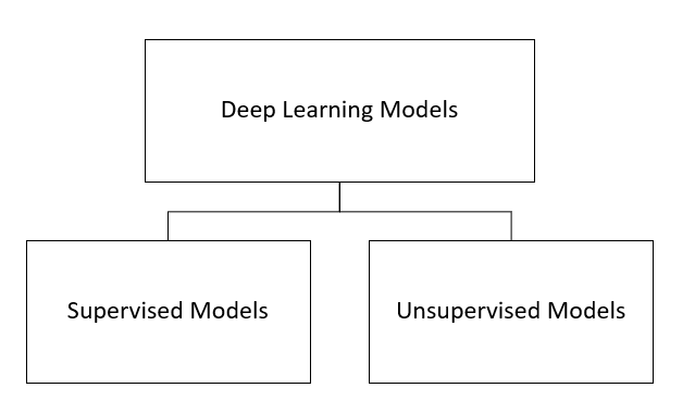
Let us first take Supervised Models, whichare trained with the examples of a particular dataset. These models are:
- Classical Neural Networks
- Convolutional Neural Networks
- Recurrent Neural Networks
Classical Neural Networks
Classical Neural Networks are also known as Multilayer perceptrons or the Perceptron Model. This model was created by American psychologist in 1958. It can also be termed as A Simple neural network. This is singular in nature and adapts to basic binary patterns with a series of inputs to simulate the learning patterns of human-brain. Its basic condition is to consist of more than 2 layers.

Application of Deep Learning in Finance
In this code below, we try to predict the direction of market movement using a set of features. Since it can either be an uptrend or downtrend it’s a binary classification problem.
# Importing the modules
import yfinance as yf
import pandas as pd
import numpy as np
import math
from sklearn.preprocessing import MinMaxScaler
from sklearn.metrics import mean_squared_error
from keras.models import Sequential
from keras.layers import Dense, Activation, Dropout
from keras.layers import LSTM
from sklearn.metrics import confusion_matrix
# Downloading GOOGLE OHLCV using yfinance
dataset = yf.download(“GOOG”, start=”2017-01-01″, end=”2019-11-30″)
# Re-adjusting OHL data using Adjusted Close
dataset[‘adjustment’] = dataset[‘Adj Close’]/dataset[‘Close’]
dataset[‘Adj Open’] = dataset[‘adjustment’] * dataset[‘Open’]
dataset[‘Adj High’] = dataset[‘adjustment’] * dataset[‘High’]
dataset[‘Adj Low’] = dataset[‘adjustment’] * dataset[‘Low’]
# The features used for classification:
# 1) Mean of Adjusted Open, High, Low and Close
OHLCV_mean = dataset[[‘Adj Open’,’Adj High’,’Adj Low’]].mean(axis = 1)
# 2) Adjusted Close
close_val = dataset[[‘Adj Close’]]
# 3) Returns of day before
returns = dataset[[‘Adj Close’]].pct_change()
# Creating a feature matrix – X – by merging all the above features
X = pd.concat([OHLCV_mean,close_val,returns],axis=1)
X.columns = [‘OHLC’,’Adj Close’,’Returns’]
# Convert the feature matrix to a numpy array
X = X.to_numpy()
# Get the corresponding binary labels for uptrend(1) or downtrend(0)
Y = (np.sign(np.roll(X[:,2],shift=-1))+1)/2
# Defining the min-max scalar for scaling the features
scaler = MinMaxScaler(feature_range=(0, 1))
# Scaling the features
X = scaler.fit_transform(X)
# Stack the label with the features
XY = np.concatenate([X,Y.reshape(-1,1)],axis=1)
# Remove all rows with either feature or label null
XY = XY[~np.isnan(XY).any(axis=1)]
# Test-Train split of the dataset
train_XY_len = int(XY.shape[0] * 0.75)
trainXY, testXY = XY[0:train_XY_len], XY[train_XY_len:]
# Separating the features and the label
# for both test and train sets
trainX = trainXY[:,:3]
trainY = trainXY[:,3]
testX = testXY[:,:3]
testY = testXY[:,3]
# Reformat or reshape test and train sets to make them compatible with
# model input stipulations
trainX = np.reshape(trainX, (trainX.shape[0], 1, trainX.shape[1]))
testX = np.reshape(testX, (testX.shape[0], 1, testX.shape[1]))
# Number of features
step_size = 3
#Define the sequential object
classifier = Sequential()
# Add LSTM later with 50 units and input size (1,3)
classifier.add(LSTM(units = 50, return_sequences = True, input_shape = (1, step_size)))
# Add dropout for regularisation
classifier.add(Dropout(0.2))
# Add another LSTM unit
classifier.add(LSTM(units = 50, return_sequences = True))
# Add dropout for regularisation
classifier.add(Dropout(0.2))
classifier.add(LSTM(units = 50, return_sequences = True))
classifier.add(Dropout(0.2))
classifier.add(LSTM(units = 50))
classifier.add(Dropout(0.2))
# Add fully connected layer with one output
classifier.add(Dense(units = 1))
# Compile the model – set loss function, optimisation algorithm and evaluation metric
model.compile(loss=’mean_squared_error’, optimizer=’adam’,metrics=[‘accuracy’])
# Train the model
model.fit(trainX, trainY, epochs=10, batch_size=1)
# Get test and train set predictions
trainPredict = model.predict(trainX)
testPredict = model.predict(testX)
# Get the confusion matrix for binary classification
confusion_matrix(testY,np.where(testPredict>0.5,1,0))
Visit QuantInsti website to read the full article:
https://blog.quantinsti.com/deep-learning-finance/
Disclosure: Interactive Brokers Third Party
Information posted on IBKR Campus that is provided by third-parties does NOT constitute a recommendation that you should contract for the services of that third party. Third-party participants who contribute to IBKR Campus are independent of Interactive Brokers and Interactive Brokers does not make any representations or warranties concerning the services offered, their past or future performance, or the accuracy of the information provided by the third party. Past performance is no guarantee of future results.
This material is from QuantInsti and is being posted with its permission. The views expressed in this material are solely those of the author and/or QuantInsti and Interactive Brokers is not endorsing or recommending any investment or trading discussed in the material. This material is not and should not be construed as an offer to buy or sell any security. It should not be construed as research or investment advice or a recommendation to buy, sell or hold any security or commodity. This material does not and is not intended to take into account the particular financial conditions, investment objectives or requirements of individual customers. Before acting on this material, you should consider whether it is suitable for your particular circumstances and, as necessary, seek professional advice.





Join The Conversation
For specific platform feedback and suggestions, please submit it directly to our team using these instructions.
If you have an account-specific question or concern, please reach out to Client Services.
We encourage you to look through our FAQs before posting. Your question may already be covered!