Autocorrelation and autocovariance are one of the most critical metrics in financial time series econometrics. Both functions are based on covariance and correlation metrics. You will learn more about them. This easy-to-learn essential guide will help you understand better about ARMA models.
- What is autocovariance?
- What is autocorrelation?
- What are the autocovariance and autocorrelation at lag zero?
- Calculation of autocovariance with an example
- Calculation of autocorrelation with an example
- Computation of autocovariance and autocorrelation in Python
- Plot the autocorrelation function in Python
- Computation of autocovariance and autocorrelation in R
- Plot the autocorrelation functions in R
- What is partial autocorrelation?
- Computation of partial autocorrelation in Python and R
You might have encountered yourself trying to learn the Autoregressive Moving Average (ARMA) model. You then started to see a lot of use of covariances and correlations, but strangely enough, you see those two words with the prefix “auto” and you get frightened!
Don’t worry, this article will help you understand their details. Just keep the focus on the article and everything will be ok!
What is autocovariance?
First, you need to understand what covariance and correlation are. Remember that covariance is applied to 2 assets. The autocovariance is the same as the covariance.
The only difference is that the autocovariance is applied to the same asset, i.e., you compute the covariance of the asset price return X with the same asset price return X, but from a previous period.
How’s that possible? Simple, check it out:

Where X and Y can be the returns of asset X and Y, respectively.
Now, the autocovariance function can be defined as:

Where:

What is autocorrelation?
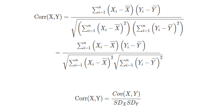
In simple terms, autocorrelation is the same as the correlation function! To be specific, autocorrelation, as the autocovariance, is applied to the same asset.
Check the difference between correlation and autocorrelation (also called serial correlation) below:

Where:

Now let’s check the autocorrelation:

Where:

.
You might ask us:
Why variance and not the multiplication of the standard deviation of the returns at the different lags?
Well, you must remember that an ARMA model is applied to stationary time series. This topic belongs to time series analysis. Consequently, it is assumed that the price returns, if stationary, have the same variance for any lag, i.e.:

What are the autocovariance and autocorrelation at lag zero?
Interesting question and simple to answer! Let’s see first for the former:

Can you guess what the last part resembles?
It is the variance of the price returns!
Consequently, the autocovariance of the returns at lag 0 is the variance of the returns.
Can you guess now what the autocorrelation of the returns would be at lag 0?Let’s use the formulas to find out:

Since we know, from the above algebraic calculation, that the covariance of the same variable is its variance, we have the following:

Consequently, the autocorrelation function for any asset price return at lag 0 is always 1.
Stay tuned for the next installment in this series to learn about calculation of the autocovariance.
Visit QuantInsti for additional insight on this topic: https://blog.quantinsti.com/autocorrelation-autocovariance/.
Disclosure: Interactive Brokers Third Party
Information posted on IBKR Campus that is provided by third-parties does NOT constitute a recommendation that you should contract for the services of that third party. Third-party participants who contribute to IBKR Campus are independent of Interactive Brokers and Interactive Brokers does not make any representations or warranties concerning the services offered, their past or future performance, or the accuracy of the information provided by the third party. Past performance is no guarantee of future results.
This material is from QuantInsti and is being posted with its permission. The views expressed in this material are solely those of the author and/or QuantInsti and Interactive Brokers is not endorsing or recommending any investment or trading discussed in the material. This material is not and should not be construed as an offer to buy or sell any security. It should not be construed as research or investment advice or a recommendation to buy, sell or hold any security or commodity. This material does not and is not intended to take into account the particular financial conditions, investment objectives or requirements of individual customers. Before acting on this material, you should consider whether it is suitable for your particular circumstances and, as necessary, seek professional advice.


Join The Conversation
For specific platform feedback and suggestions, please submit it directly to our team using these instructions.
If you have an account-specific question or concern, please reach out to Client Services.
We encourage you to look through our FAQs before posting. Your question may already be covered!