Excerpt
What is Time Series and Time Series Analysis
In simple words, Time Series is a sequence of observations over time, which are usually spaced at regular intervals. To support the statement, here are some of the examples of Time Series:
- Daily stock prices for the last 5 years
- 1-minute stock price data for the last 90 days
- Quarterly revenues of a company over the last 10 years
- Monthly car sales of an automaker for the last 3 years
- The annual unemployment rate of a state in the last 50 years
Coming to Time Series analysis, it simply implies identifying those methods which help in the analysis of Time Series data.
The main aim of the Time Series Analysis is to develop those models that best capture or describe the Time Series or data set. Also, this leads to an understanding of the underlying causes of the dataset to help you create meaningful and accurate forecasts.
Also, there are few types of Time Series which we will see ahead.
Types of Time Series
Let us now look at the types of Time Series that a dataset can belong to:
- Univariate & Multivariate
- Stationary & Non-Stationary
Univariate & Multivariate
A Univariate Time Series refers to the set of observations over time of a single variable. One important thing to note here is that this type always has the time as an implicit variable. And, if the data points are equally spaced, then the time variable need not be explicitly given. This type helps you decide as to how the dependent variable (price values) differs with regard to time, which is the independent variable.
For example, a Company A’s stock prices’ data is taken out for the past two years with stock price mentioned for every month of every year. Here, let us assume that the stock prices are in a particular range for the months of December and January.
A Multivariate Time Series refers to the set of observations over time of several variables and not one. In this type, each variable is dependent not only on one type of equispaced data but also on other variables apart from it.
For example, the same company A’s stock prices are not only dependent on time which was set at every month of every year, but also on other variables like a fashion trend, occasion, etc.
Stationary & Non-Stationary Time Series
Stationary Time Series
Defining a Stationary Time Series, it is the one where the mean and the variance are both constant over time. In other words, it is the one whose properties do not depend on the time at which the series is observed. Thus, the Time Series is a flat series without trend, with constant variance over time, a constant mean, a constant autocorrelation and no seasonality. This makes a Stationary Time Series easy to predict.
Non-Stationary
A Non-Stationary Time Series is one where either mean or variance or both are not constant over time.
There are different tests that can be used to check whether a given Time Series is Stationary:
- Autocorrelation function (ACF) test
- Partial autocorrelation function (PACF) test
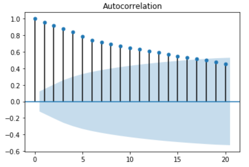
Autocorrelation function (ACF) Test – The Autocorrelation function checks for correlation between two different data points of a Time Series separated by a lag “h”. For example, the ACF will check for correlation between points #1 and #2, #2 and #3 etc. Similarly, for lag 3, the ACF function will check between points #1 and #4, #2 and #5, #3 and #6 etc.
Autocorrelation function test is mainly used for two reasons:
- For detecting non-randomness in the data and
- For identifying the appropriate time series model for the particular dataset.
So an Autocorrelation Function Test, therefore, is important for providing accurate results.
Python code for ACF-
from matplotlib import pyplot
from statsmodels.graphics.tsaplots import plot_acf
import yfinance as yf
tesla = yf.download(‘TSLA’,’2019-01-27′, ‘2020-02-11’)
plot_acf(tesla[‘Close’], lags=20)
pyplot.show()
Python code – ACF.py hosted with ❤ by GitHub
Once you run the Python code above, you get a 2D plot of the autocorrelation with first 20 lags:

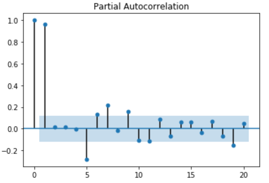
Partial autocorrelation function (PACF) – In some cases, the effect of autocorrelation at smaller lags will have an influence on the estimate of autocorrelation at longer lags. For example, a strong lag one, can cause an autocorrelation with lag three. The Partial autocorrelation function (PACF) removes the effect of shorter lag autocorrelation from the correlation estimate at longer lags.
Python code for PACF-
from statsmodels.graphics.tsaplots import plot_pacf
plot_pacf(tesla[‘Close’], lags=20)
pyplot.show()
Python code – ACF.py hosted with ❤ by GitHub
Running the code above brings a 2D representation of the data with partial autocorrelation for the first 20 lags:

The values of ACF and PACF each vary between plus and minus one. When the values are closer to plus or minus one, it indicates a strong correlation. Moreover, it is a must to note that, if the Time Series is Stationary, the ACF will drop to zero relatively quickly. Whereas, the ACF of Non-Stationary Time Series will decrease slowly. Also, with the ACF graph, we can conclude that the given Time Series is Non-Stationary.
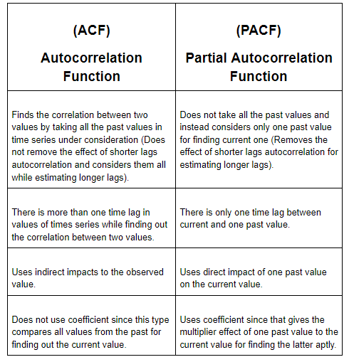
Okay now! Let us explore some differences between ACF and PACF for an easy understanding:

To download the Python code and read the full article, visit QuantInsti Blog: https://blog.quantinsti.com/time-series-analysis/
Disclosure: Interactive Brokers Third Party
Information posted on IBKR Campus that is provided by third-parties does NOT constitute a recommendation that you should contract for the services of that third party. Third-party participants who contribute to IBKR Campus are independent of Interactive Brokers and Interactive Brokers does not make any representations or warranties concerning the services offered, their past or future performance, or the accuracy of the information provided by the third party. Past performance is no guarantee of future results.
This material is from QuantInsti and is being posted with its permission. The views expressed in this material are solely those of the author and/or QuantInsti and Interactive Brokers is not endorsing or recommending any investment or trading discussed in the material. This material is not and should not be construed as an offer to buy or sell any security. It should not be construed as research or investment advice or a recommendation to buy, sell or hold any security or commodity. This material does not and is not intended to take into account the particular financial conditions, investment objectives or requirements of individual customers. Before acting on this material, you should consider whether it is suitable for your particular circumstances and, as necessary, seek professional advice.


Join The Conversation
For specific platform feedback and suggestions, please submit it directly to our team using these instructions.
If you have an account-specific question or concern, please reach out to Client Services.
We encourage you to look through our FAQs before posting. Your question may already be covered!